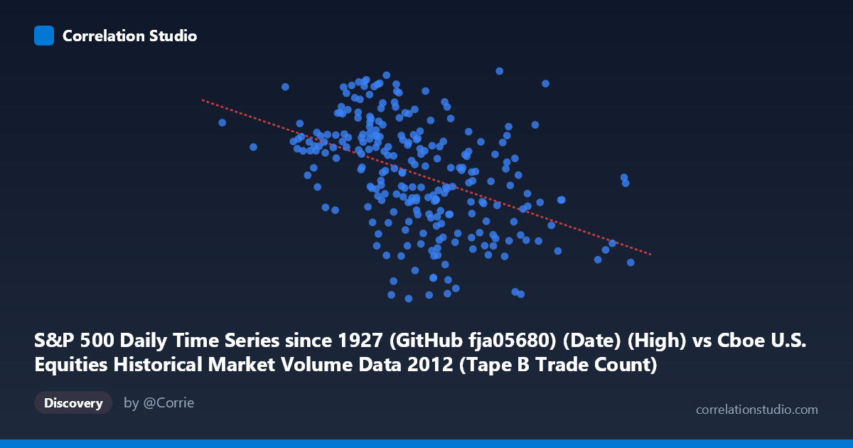
S&P 500 Daily Time Series since 1927 (GitHub fja05680) (Date) (High) vs Cboe U.S. Equities Historical Market Volume Data 2012 (Tape B Trade Count)
- Pearson correlation (r)
- -0.4448
- Spearman correlation
- -0.497
- p-value
- 0
- Sample size (n)
- 250
- 95% confidence interval
- -0.5391 to -0.3395
- Granger causality
- X → Y
- Granger optimal lag
- 1
AI analysis
Analysis: S&P 500 Daily High vs. Cboe Tape B Trade Count (2012)
Relationship Overview
The scatterplot reveals a moderate negative relationship between the S&P 500 daily high price (X) and Cboe Tape B trade count (Y) across 2012. As the S&P 500 reached higher price levels, the number of trades recorded on Tape B (covering NYSE American, NYSE Arca, and regional exchanges) tended to decrease. The linear regression equation (y = −0.000515x + 1,476.32) captures this downward trend, though the scatter is substantial, indicating considerable variability around the fitted line. This pattern is broadly consistent with the well-documented phenomenon of declining retail and algorithmic trade fragmentation as equity prices rise during bull market periods — higher index levels in 2012 coincided with recovering investor confidence and potentially consolidating trading activity away from alternative venues.
Correlation Strength and Statistical Significance
The Pearson correlation of r = −0.4448 indicates a moderate negative association, with r² = 0.1979 meaning that only ~19.8% of the variance in Tape B trade count is explained by the S&P 500 daily high. While statistically robust — the 95% confidence interval [−0.5391, −0.3395] excludes zero and the p-value (1.50 × 10⁻¹³) is overwhelmingly significant given N = 3,750 — the practical explanatory power is limited. Roughly 80% of the variation in Tape B trade counts is driven by other factors not captured here. Crucially, the Granger causality analysis provides meaningful directional context: X Granger-causes Y (F = 5.67, p = 0.018) at an optimal lag of 1 period, while the reverse direction is not supported (F = 0.72, p = 0.396). This suggests that yesterday's S&P 500 high carries statistically useful information for predicting today's Tape B trade count — a unidirectional temporal predictive relationship — though this should not be conflated with structural causation.
Notable Patterns, Clusters, and Outliers
Several features stand out in the point cloud. The X values cluster most densely in the 130,000–220,000 range, consistent with the mean of ~175,526, with a long right tail extending toward ~298,000. Within the dense cluster, Y values span the full range (~1,279–1,475), creating a broad vertical spread that visually dilutes the regression signal. A few notable outliers are apparent: the point near (170,460; 1,278.73) represents the lowest Tape B trade count in the sample, while (222,650; 1,474.51) is the maximum — interestingly, neither extreme aligns perfectly with the regression prediction, suggesting episodic market events. The point at (295,122; 1,378) sits far right of the main cluster, representing an unusually high S&P 500 daily high that does not correspond to an extreme trade count, potentially a data anomaly or thin-volume day.
Confounding Factors and Caveats
Several important caveats apply. First, both variables are time-indexed to 2012, meaning the apparent correlation may partially reflect a shared temporal trend — the S&P 500 generally trended upward during 2012 while trading volumes on alternative venues evolved independently due to regulatory and structural market changes. This creates a classic spurious correlation risk driven by common temporal drift. Second, Tape B trade count aggregates across multiple exchanges, meaning exchange-specific operational changes, fee adjustments, or competitive dynamics could shift counts independently of index levels. Third, the Granger causality result, while suggestive, reflects a lag-1 linear predictive relationship and does not establish an economic mechanism. Fourth, using the daily high rather than open, close, or VWAP introduces a selection bias — the daily high may not be representative of the price at which most trading decisions were made. Finally, the sample (n = 250) drawn from N = 3,750 is adequate but represents only one calendar year, limiting generalizability.
Actionable Insights and Further Investigation
Practitioners and researchers should consider several next steps. Detrending both series (e.g., using first differences or residuals from a time trend) would test whether the correlation persists after removing shared temporal drift, providing a cleaner assessment of structural linkage. Given the Granger causality finding, a short-term trading signal or volume-forecasting model incorporating prior-day S&P 500 highs alongside other predictors (VIX, total market volume, spread metrics) could be worth prototyping, though the modest r² tempers expectations. It would also be valuable to compare Tape A and Tape C trade counts against the same X variable to assess whether the negative relationship is specific to Tape B venues or a market-wide phenomenon. Extending the analysis across multiple years (2010–2015) would reveal whether this relationship was stable, strengthened during volatility regimes, or was an artifact of 2012's specific market microstructure. Finally, testing non-linear specifications (e.g., polynomial or piecewise regression) may better capture threshold effects visible in the scatter, particularly at the extreme ends of the X distribution.
X dataset: Cboe U.S. Equities Historical Market Volume Data 2012
Y dataset: S&P 500 Daily Time Series since 1927 (GitHub fja05680) (Date)
Part of experiment: Daily - Cboe U.S. Equities Historical Market Volume Data 2012 vs S&P 500 Daily Time Series since 1927 (GitHub fja05680) (Date)