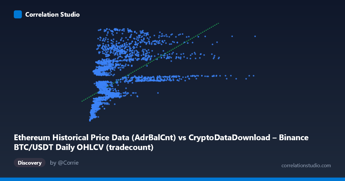
Ethereum Historical Price Data (AdrBalCnt) vs CryptoDataDownload – Binance BTC/USDT Daily OHLCV (tradecount)
- Pearson correlation (r)
- 0.5658
- Spearman correlation
- 0.7894
- p-value
- 0
- Sample size (n)
- 3191
- 95% confidence interval
- 0.5417 to 0.5889
- Granger causality
- None
- Granger optimal lag
- 10
- Time coverage
- 2017-08-17 to 2026-05-20
AI analysis
Analysis of Scatterplot Relationship
1. Overview of the Relationship
The scatterplot depicts a positive but moderate association between the X variable (labeled as an Ethereum "AdrBalCnt" metric, though contextually behaving like a price/volume-scaled figure) and Y (labeled as Binance BTC/USDT trade count). Despite the confusing column labels, the data show a classic concave/decelerating pattern: Y rises steeply as X increases from near-zero, then the rate of increase flattens out at higher X values. This is visible in the sample points — small X values (hundreds to low thousands) correspond to a wide spread of Y values, including some very high ones (e.g., X=919,594 → Y=159M), while large X values (millions) don't proportionally produce the highest Y values. This saturating shape is the hallmark of a logarithmic or power-law relationship rather than a straight line.
2. Strength, Direction, and Statistical Confidence
The Pearson correlation (r = 0.566) indicates a moderate positive linear relationship, but r² = 0.320 means only 32% of the variance in Y is explained by X in a linear framework — leaving roughly two-thirds of Y's variability unaccounted for by this single predictor. The 95% CI [0.542, 0.589] is tight, and p ≈ 0 confirms this correlation is highly statistically significant and not due to chance — with n=3,191, even modest correlations are detected reliably. However, statistical significance ≠ practical strength: a moderate r² leaves substantial room for other drivers of Y. Critically, the Granger causality tests show no significant predictive direction either way (X→Y: p=0.255; Y→X: p=0.801) at the optimal 10-period lag. This means neither series reliably forecasts the other over time — the correlation is likely contemporaneous/structural (e.g., both driven by common market conditions) rather than one causing or leading the other.
3. Notable Patterns and Non-linearity
The most important pattern is the fan/funnel shape: variance in Y is much larger at low-to-mid X values than the linear fit assumes, and the relationship bends — consistent with the note that Spearman ρ exceeds Pearson r, confirming a monotonic but non-linear relationship. A log-transform of X (or a power/log model) would likely fit substantially better than the current linear equation (y = 12.7x + 52.36M). There also appear to be extreme outliers/high-leverage points — X's max (15.36M) is nearly 7 standard deviations above its mean (1.97M ± 2.24M), suggesting a heavy right-skew or a few extraordinary events (likely bull-market peaks) pulling the linear fit's slope.
4. Caveats and Confounders
Several caveats limit interpretation: - Label inconsistency: the axis descriptions cross-reference mismatched datasets (Ethereum "AdrBalCnt" on X but described under a BTC/USDT OHLCV dataset; "tradecount" on Y attributed to Ethereum data) — this suggests possible data-pipeline mislabeling that should be verified before drawing domain conclusions. - Time-series autocorrelation: both series span 2017–2026 and are likely trending together due to shared crypto market cycles (bull/bear phases), inflating the correlation without implying direct causation — classic spurious correlation via common trend risk. - Skewed distributions: heavy right-skew in both X and Y (means far exceed medians implied by ranges) means Pearson r may be distorted by outliers; robust/rank-based correlation (Spearman) is more trustworthy here. - Non-stationarity: crypto metrics like trade count and address balances are typically non-stationary (trending, volatile), which can bias both Pearson correlation and Granger tests unless differenced/detrended first.
5. Suggestions for Further Investigation
1. Verify data labeling — confirm which metrics X and Y actually represent, since the current labels are self-contradictory. 2. Refit with non-linear models — try log-log or log-linear regression given the concave pattern and Spearman/Pearson divergence; this should raise explained variance substantially. 3. Detrend/difference the series before re-running Granger causality, since raw non-stationary series can mask or distort lead-lag relationships. 4. Segment by market regime (bull vs. bear periods) to check if the X-Y relationship is regime-dependent rather than constant across the full 2017–2026 window. 5. Investigate outliers at extreme X values to determine if they represent legitimate market events or data errors, since they exert disproportionate influence on the linear fit.
X dataset: CryptoDataDownload – Binance BTC/USDT Daily OHLCV
Y dataset: Ethereum Historical Price Data
Part of experiment: Bitcoin - CryptoDataDownload – Binance BTC/USDT Daily OHLCV vs Ethereum Historical Price Data