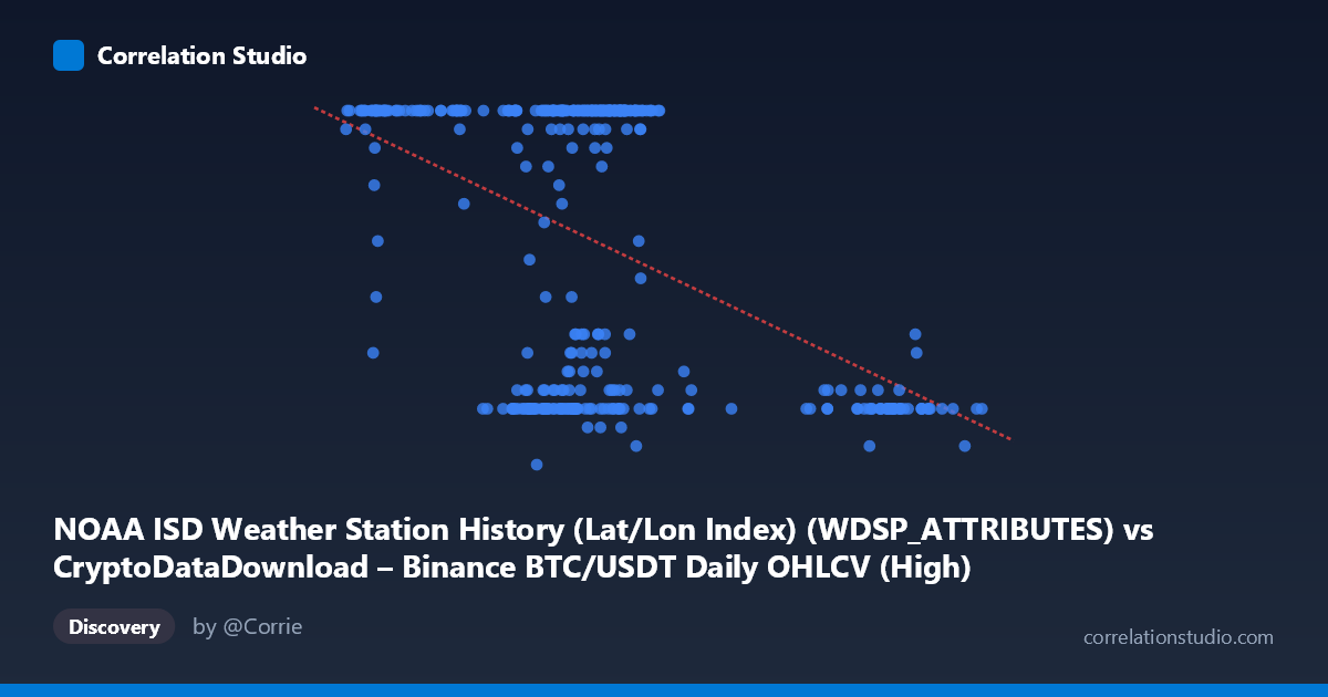
NOAA ISD Weather Station History (Lat/Lon Index) (WDSP_ATTRIBUTES) vs CryptoDataDownload – Binance BTC/USDT Daily OHLCV (High)
- Pearson correlation (r)
- -0.4675
- Spearman correlation
- -0.2951
- p-value
- 0
- Sample size (n)
- 355
- 95% confidence interval
- -0.5451 to -0.382
- Granger causality
- None
- Granger optimal lag
- 1
- Time coverage
- 2024-01-01 to 2024-12-31
AI analysis
Analysis of Scatterplot Relationship
1. Overview of the Visualization
The scatterplot displays a moderate negative relationship between the two variables, with a correlation coefficient of r = -0.4675. Visually, the data shows a dense concentration of points in the X range of roughly 50,000–75,000, with Y values clustering heavily at the upper bound (around 24) and a secondary cluster near the lower bound (8-12). This bimodal distribution in Y, rather than a smooth continuous spread, is a striking feature — the data does not resemble a classic linear cloud but rather two horizontal bands with a transitional/declining relationship as X increases beyond ~70,000.
2. Strength, Direction, and Statistical Confidence
The correlation is negative and moderate in strength (r = -0.4675), meaning that as X increases, Y tends to decrease. However, r² = 0.2185 indicates that only about 21.9% of the variance in Y is explained by X — meaning nearly 78% of Y's variability is driven by other factors entirely. The 95% confidence interval [-0.5451, -0.3820] is reasonably tight and does not cross zero, and the p-value of ~0 confirms this correlation is statistically significant and not due to chance, given the sample size (n=355). That said, statistical significance here reflects sample size more than practical predictive power — r² of 0.22 is a weak-to-moderate explanatory relationship in practice. Critically, the Granger causality tests show no significant predictive direction in either direction (X→Y: p=0.708; Y→X: p=0.233). This strongly suggests the correlation is not driven by one variable temporally leading the other — it may instead reflect a shared underlying trend, seasonal confound, or coincidental co-movement rather than a causal or forecastable dynamic.
3. Notable Patterns and Outliers
The most striking feature is the ceiling effect at Y=24 — a large number of points sit exactly at this value across a wide range of X (40,000–75,000), suggesting this may be a capped, saturated, or discretized variable (e.g., a maximum recorded value or rounding artifact) rather than a natural continuous measurement. Additionally, there's a distinct low-Y cluster (Y ≈ 7-12) appearing mostly at higher X values (60,000-100,000+), including some clear outliers like (98564, 8) and (91449.99, 9) at the high end of X. This creates the appearance of a negative trend, but it's driven largely by two separate clusters rather than a smooth linear decay — suggesting the relationship may be better characterized as threshold-based or regime-switching rather than linear.
4. Confounding Factors and Caveats
Given the dataset labeling irregularities (X labeled as a Weather Station index but describing BTC/USDT OHLCV data, and Y labeled as OHLCV "High" but appearing to describe weather-like data), there appears to be a metadata/column mismatch in this dataset pairing. This is a serious caveat — the "relationship" may be an artifact of merging two unrelated time series (crypto price data and weather station data) that happen to share a time index but have no substantive real-world connection. Spurious correlation due to shared time trends (e.g., both variables trending across 2024) is highly plausible, especially absent Granger causality. The ceiling/floor clustering in Y also suggests potential data quality issues (capping, categorical encoding, or measurement artifacts) rather than a clean continuous variable.
5. Recommendations for Further Investigation
Given the mismatched metadata, the first step should be verifying data provenance and correct column-to-source mapping before drawing any substantive conclusions. If the variables are confirmed as intended, I recommend: (a) investigating the bimodal/capped structure in Y — determine why so many values sit at exactly 24, and consider treating this as a censored or categorical variable rather than continuous; (b) testing for non-linear or regime-based models (e.g., piecewise regression, clustering analysis) rather than relying on linear r²; (c) checking for a shared time trend or seasonal confound by detrending both series and re-testing correlation; and (d) given the lack of Granger causality, avoid using either variable to forecast the other, and instead search for a plausible third-variable driver (e.g., calendar season, market cycle) that may explain the co-movement.
X dataset: CryptoDataDownload – Binance BTC/USDT Daily OHLCV
Y dataset: NOAA ISD Weather Station History (Lat/Lon Index)
Part of experiment: Bitcoin - CryptoDataDownload – Binance BTC/USDT Daily OHLCV vs NOAA ISD Weather Station History (Lat/Lon Index)