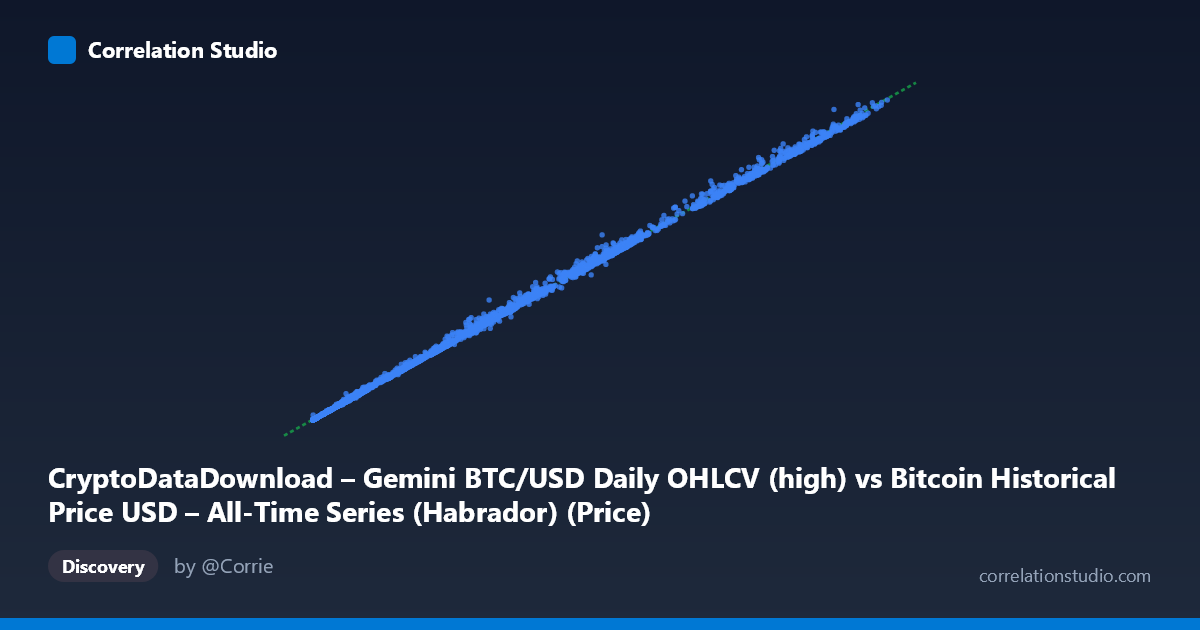
CryptoDataDownload – Gemini BTC/USD Daily OHLCV (high) vs Bitcoin Historical Price USD – All-Time Series (Habrador) (Price)
- Pearson correlation (r)
- 0.9997
- Spearman correlation
- 0.9997
- p-value
- 0
- Sample size (n)
- 3856
- 95% confidence interval
- 0.9996 to 0.9997
- Granger causality
- None
- Granger optimal lag
- 10
- Time coverage
- 2015-10-08 to 2026-04-28
- Recomputed on refreshed data
- 2026-10-23 (r was 0.9997)
AI analysis
Analysis: Bitcoin Price Cross-Reference (Habrador vs. Gemini BTC/USD)
1. What the visualization reveals
The scatterplot shows an almost perfectly linear relationship between two Bitcoin price series spanning from late 2015 through early 2026. Points trace a tight diagonal line from near-zero (hundreds of dollars) through tens of thousands of dollars, up to the ~$120,000+ range, with virtually no dispersion around the fitted line. This pattern is consistent with two data sources measuring the same underlying asset price at the same points in time, rather than two genuinely independent variables that happen to move together.
2. Strength, direction, and what it means practically
The correlation is essentially maximal (r = 0.9997, r² = 0.9993), meaning 99.93% of the variance in the Gemini "high" price is explained by the Habrador price series (and vice versa). The 95% CI [0.9996, 0.9997] is extremely narrow, and the p-value of ~0 confirms this relationship is not a statistical artifact — with n = 3,856 paired daily observations, there is no meaningful uncertainty about the strength of this association. The regression slope of 1.016 with a small positive intercept (138.9) indicates the two series are nearly 1:1, with Gemini values running slightly higher on average — plausible given it's a "high" price versus what may be a close/average price in the other source. Notably, the Granger causality tests show no significant predictive direction in either direction (p ≈ 0.20 both ways). This is the key practical takeaway: neither series "leads" the other in time. This is exactly what you'd expect if both columns describe the same market event (BTC price on a given day) rather than two causally linked but distinct phenomena — there's no lead/lag structure to exploit for forecasting one from the other.
3. Notable patterns, clusters, and outliers
The sample points show the expected exponential/multi-cycle clustering typical of Bitcoin's history: dense clusters at low values (sub-$10,000, corresponding to 2015–2019) and progressively sparser, higher-magnitude points reflecting the 2020–2021, 2023–2024, and 2025–2026 bull runs. A few sample rows show larger absolute deviations at higher price levels (e.g., 78,816 vs. 84,127; 108,530 vs. 112,641; 90,120 vs. 92,798) — differences of several thousand dollars. This is likely heteroscedastic: absolute deviations grow with price level even though relative deviations stay small, which is consistent with these being high/close price spreads during volatile trading days rather than the same instantaneous price point.
4. Confounding factors and caveats
This is not really a "correlation between two independent variables" — it's closer to a consistency/reconciliation check between two records of the same asset's price history, likely differing by exchange (Gemini vs. an aggregate/all-time series) and possibly by price field (high vs. close/average). Key caveats: (a) both series share the same underlying market volatility and macro trends (halving cycles, regulatory news, liquidity shocks), so the "relationship" is largely definitional rather than causal; (b) the mismatch in population size (N=4,267 vs. paired n=3,856) suggests ~411 unmatched dates — possibly exchange downtime, listing gaps, or date-alignment issues that could bias the sample if missingness isn't random; (c) heteroscedasticity (larger absolute gaps at higher prices) violates constant-variance assumptions of simple linear regression, though this barely affects r² given the scale of the relationship.
5. Actionable insights and further investigation
Given the near-identity relationship, this pair is best used as a data validation/reconciliation tool — flagging days where the two sources diverge by more than a few percent (e.g., the 78,816/84,127 and 108,530/112,641 pairs) to investigate exchange-specific volatility, data entry errors, or timestamp misalignment (e.g., UTC vs. exchange-local close times). Rather than modeling one series as a function of the other for forecasting, analysts should treat persistent gaps as the signal of interest — e.g., building a spread/basis series (Y−X or Y/X) and analyzing that for exchange premium patterns, arbitrage windows, or liquidity differences. The absence of Granger causality confirms there's no forecasting edge in lead-lag terms; effort is better spent reconciling the ~10% of records that didn't merge (N vs. n gap) and auditing outlier days for data quality rather than treating this as a predictive relationship.
X dataset: Bitcoin Historical Price USD – All-Time Series (Habrador)
Y dataset: CryptoDataDownload – Gemini BTC/USD Daily OHLCV
Part of experiment: Bitcoin - Bitcoin Historical Price USD – All-Time Series (Habrador) vs CryptoDataDownload – Gemini BTC/USD Daily OHLCV