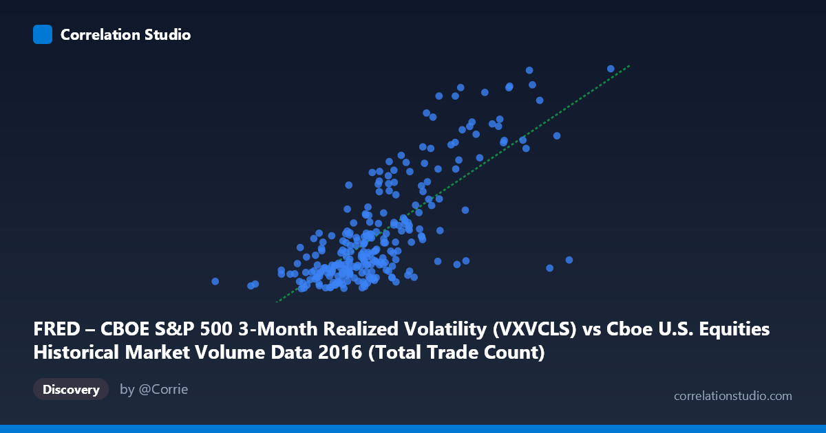
FRED – CBOE S&P 500 3-Month Realized Volatility (VXVCLS) vs Cboe U.S. Equities Historical Market Volume Data 2016 (Total Trade Count)
- Pearson correlation (r)
- 0.7494
- Spearman correlation
- 0.6957
- p-value
- 0
- Sample size (n)
- 252
- 95% confidence interval
- 0.6897 to 0.799
- Granger causality
- None
- Granger optimal lag
- 1
AI analysis
Analysis: CBOE S&P 500 3-Month Realized Volatility vs. Total Trade Count (2016)
Relationship Overview The scatterplot reveals a meaningful positive relationship between CBOE S&P 500 3-Month Realized Volatility (VXVCLS) and total trade count in U.S. equity markets throughout 2016. As volatility increases, trading activity — measured by total trade count — tends to rise correspondingly. This is consistent with well-established market microstructure theory: elevated uncertainty and price dispersion incentivize both hedging activity and speculative trading, driving higher transaction volumes. The linear regression equation (y = 4.30266E-06x + 7.837) captures this upward trend, though the relatively shallow slope suggests that trade count responds gradually rather than explosively to incremental volatility increases.
Correlation Strength and Statistical Significance The Pearson correlation of r = 0.7494 indicates a moderately strong positive association. More precisely, r² = 0.5616, meaning that approximately 56.2% of the variance in total trade count is explained by realized volatility — a substantial explanatory share, but also a reminder that nearly 44% of variation lies elsewhere. The 95% confidence interval of [0.6897, 0.7990] is notably tight, reflecting the large paired sample (n = 252, drawn from N = 3,622), and the p-value of effectively zero confirms this relationship is not a statistical artifact. However, the Granger causality tests yield no significant directional predictive relationship in either direction (X→Y: F = 0.547, p = 0.460; Y→X: F = 0.135, p = 0.714). This is a critical nuance: while the two variables are strongly correlated contemporaneously, neither reliably predicts the other with a one-period lag. The relationship appears to be largely synchronous rather than temporally sequential, which limits its utility for short-term forecasting.
Patterns, Clusters, and Outliers The scatterplot exhibits a relatively coherent linear band across the mid-range of X values (roughly 1,900,000–2,700,000), where most observations cluster. However, several notable features stand out. At the high end — X values above ~3,000,000 and especially near 3,594,823 — there are clear high-leverage outliers with correspondingly elevated Y values (e.g., ~26.71), likely corresponding to specific high-volatility episodes in 2016 such as Brexit (June) or the U.S. election (November). At the low end, values like (1,722,715, 15.09) anchor the bottom of the distribution. There is also visible heteroscedasticity: variance in Y appears to fan outward as X increases, suggesting the relationship becomes less precise under high-volatility conditions — a pattern that a simple linear model may underfit.
Confounding Factors and Caveats Several important caveats temper interpretation. First, both variables are likely driven by common exogenous shocks (macroeconomic announcements, geopolitical events, Federal Reserve decisions) rather than one causing the other — consistent with the failed Granger tests. Second, day-of-week and seasonal effects in equity trading volumes could introduce autocorrelation that inflates apparent correlation. Third, the dataset covers only a single calendar year (2016), which included unusual market-moving events; results may not generalize to other periods. Fourth, the axes may be partially reversed in labeling (the dataset descriptions suggest X and Y source labels are swapped), which warrants verification before drawing directional conclusions. Finally, realized volatility is a backward-looking measure, while trade counts reflect real-time decisions — their contemporaneous alignment may reflect a common driver rather than any direct mechanism.
Actionable Insights and Further Investigation Practitioners monitoring market liquidity should treat elevated VXVCLS readings as a concurrent signal of heightened trading activity, useful for capacity planning, execution cost modeling, and risk management, even if it cannot be used to predict next-day trade counts. For further investigation, several avenues are promising: (1) extend the analysis across multiple years to test whether r² stability holds in low-volatility regimes (e.g., 2017); (2) decompose trade count by exchange or trade type (lit vs. dark) to identify whether the correlation is concentrated in specific venues; (3) introduce additional covariates — VIX term structure, macroeconomic surprise indices, or Fed meeting dates — to reduce the unexplained 44% variance; and (4) test non-linear models (e.g., log-log or piecewise regression) given the apparent heteroscedasticity, which may improve fit at volatility extremes.
X dataset: Cboe U.S. Equities Historical Market Volume Data 2016
Y dataset: FRED – CBOE S&P 500 3-Month Realized Volatility
Part of experiment: Daily - Cboe U.S. Equities Historical Market Volume Data 2016 vs FRED – CBOE S&P 500 3-Month Realized Volatility