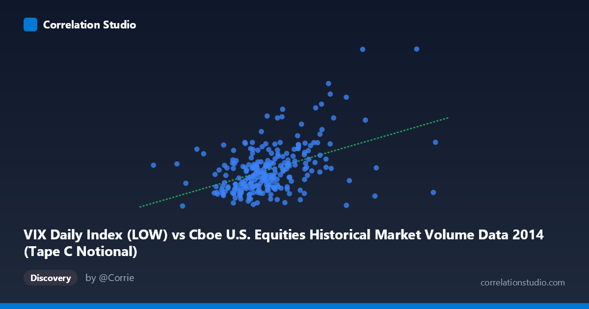
VIX Daily Index (LOW) vs Cboe U.S. Equities Historical Market Volume Data 2014 (Tape C Notional)
- Pearson correlation (r)
- 0.4514
- Spearman correlation
- 0.4054
- p-value
- 0
- Sample size (n)
- 252
- 95% confidence interval
- 0.3472 to 0.5446
- Granger causality
- None
- Granger optimal lag
- 1
AI analysis
Scatterplot Analysis: VIX Tape C Notional vs. VIX Daily Index Low
Relationship Overview
The scatterplot reveals a moderate positive relationship between the Cboe U.S. Equities Historical Market Volume (VIX Daily Index Low, X-axis) and the VIX Daily Index Tape C Notional values (Y-axis) across the 2014 trading year. The linear regression equation (y = 1.06E-09x + 8.476) confirms that as market volume increases, VIX-related notional values tend to rise as well. This is broadly intuitive: periods of elevated market activity and trading volume tend to coincide with heightened volatility expectations, which would naturally be reflected in VIX-linked products. However, the relationship is far from deterministic, and the scatterplot shows considerable dispersion around the regression line.
Correlation Strength and Statistical Significance
With r = 0.4514, the correlation is statistically significant (p = 4.685E-14) but only moderately strong. The R² of 0.2038 is the most important framing here — it means that only ~20% of the variance in Tape C Notional is explained by the VIX Low, leaving roughly 80% attributable to other factors entirely. The 95% confidence interval for r [0.3472, 0.5446] is reasonably narrow, suggesting the estimate is stable, but it confirms that even the upper bound of plausible correlation falls well short of a strong relationship. Critically, the Granger causality tests find no significant predictive directionality in either direction (X→Y: F = 0.0075, p = 0.931; Y→X: F = 0.0815, p = 0.776). This means that knowing today's market volume does not help predict tomorrow's VIX notional, and vice versa — the correlation observed is contemporaneous, not predictive, which substantially limits its practical utility for forecasting.
Notable Patterns and Outliers
Several features stand out in the data. The bulk of observations cluster in a relatively dense band between X values of ~3.5B–5.5B and Y values of ~11–16, forming the core of the distribution. However, there are clear outliers that warrant attention: - A striking point near (7.18B, 24.61) sits far from the main cluster, representing an extreme combination of high volume and very high VIX notional — likely corresponding to a specific high-volatility event day in 2014. - A point near (6.77B, 10.34) is anomalous in the opposite Y-direction — very high volume but unusually low VIX notional — suggesting a day of heavy trading activity without corresponding volatility premiums. - Points near X = 1.96B (minimum, far left) and X = 9.0B (maximum) represent tail-end trading days and appear isolated from the core cluster.
These outliers disproportionately influence the regression line and correlation coefficient, and their removal could meaningfully shift the estimated r.
Confounding Factors and Caveats
Several important caveats apply. First, there is a variable alignment concern: the X-axis is labeled as "VIX Daily Index (LOW)" from the market volume dataset, while the Y-axis is "Tape C Notional" from the VIX dataset — this cross-labeling suggests these may not be the most natural pairing, and the relationship may partly reflect dataset construction artifacts rather than a true economic signal. Second, 2014 was a relatively contained volatility year with notable spikes (e.g., October 2014 market correction), meaning the observed correlation may be period-specific and not generalizable. Third, Tape C covers NYSE-listed securities only, so volume from other tapes or venues could be a confound. Finally, the sample of n = 252 trading days from a population of N = 3,686 introduces sampling considerations, though the p-value suggests the sample is sufficiently powered.
Actionable Insights and Further Investigation
Given the moderate correlation and lack of Granger causality, practitioners should avoid using either variable as a standalone predictor of the other. Instead, several follow-up analyses are recommended: (1) Investigate the extreme outliers — identifying the specific dates and events behind the (7.18B, 24.61) and (6.77B, 10.34) anomalies could yield meaningful market microstructure insights; (2) Segment the analysis by market regime (e.g., low-VIX vs. high-VIX periods) to test whether the correlation strengthens during stress periods; (3) Incorporate all Tape segments (A, B, C) to assess whether Tape C is representative of broader market behavior; and (4) Extend the time series beyond 2014 to test whether this relationship is structurally stable or an artifact of one calendar year's dynamics. A non-linear regression or quantile regression approach may also better capture the apparent heteroscedasticity visible in the scatterplot.
X dataset: Cboe U.S. Equities Historical Market Volume Data 2014
Y dataset: VIX Daily Index
Part of experiment: Daily - Cboe U.S. Equities Historical Market Volume Data 2014 vs VIX Daily Index