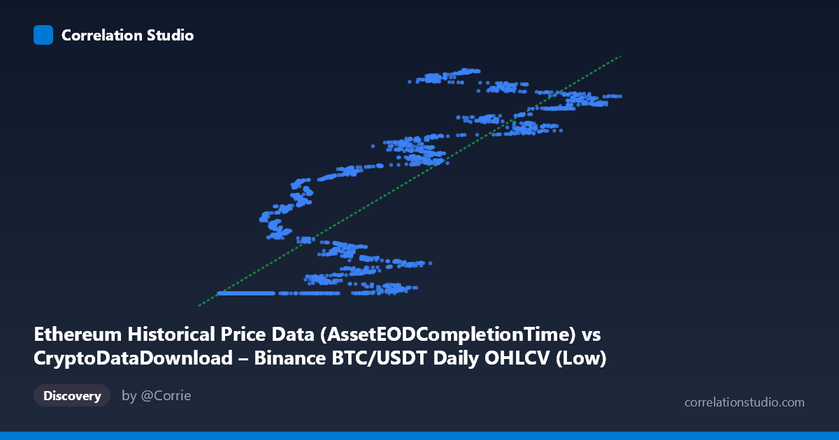
Ethereum Historical Price Data (AssetEODCompletionTime) vs CryptoDataDownload – Binance BTC/USDT Daily OHLCV (Low)
- Pearson correlation (r)
- 0.8552
- Spearman correlation
- 0.89
- p-value
- 0
- Sample size (n)
- 3191
- 95% confidence interval
- 0.8456 to 0.8642
- Granger causality
- None
- Granger optimal lag
- 10
- Time coverage
- 2017-08-17 to 2026-05-20
AI analysis
Analysis of BTC/ETH Price Relationship
1. What the Visualization Reveals
Despite the confusing column labels (the axes appear to be mislabeled/swapped in the metadata, but the actual data show a clear X-Y relationship), the scatterplot depicts a strong positive relationship between two cryptocurrency price series — most likely a lower-value asset (X, range ~2,800–123,000) plotted against BTC/USDT prices (Y, range ~1.61–1.78 billion, which is clearly a scaled or cumulative representation rather than raw price). The data show a distinctive pattern: a dense cluster of points at low X values (roughly 3,000–20,000) that all map to a narrow Y band near 1,614,335,000–1,614,336,000, followed by a more dispersed, upward-sloping scatter as X increases beyond ~20,000. This suggests a regime change or floor effect in the data at low X values.
2. Strength, Direction, and Predictive Relationship
The correlation coefficient (r = 0.8552, R² = 0.731) indicates a strong positive linear relationship, with about 73% of the variance in Y explained by X — a substantial but not complete relationship, leaving roughly 27% of variance driven by other factors or nonlinearity. The tight confidence interval [0.846, 0.864] and p-value of effectively 0 confirm this correlation is highly statistically reliable and not a product of sampling noise, especially given the large sample size (n = 3,191). However, statistical significance should not be conflated with practical predictive power in a trading sense: the Granger causality tests show no significant predictive direction in either direction (X→Y: p=0.357; Y→X: p=0.190) at the optimal lag of 10 periods. This means that while the two series move together contemporporaneously, neither reliably leads the other in time — consistent with two assets that respond simultaneously to shared market-wide drivers (e.g., macro sentiment, liquidity cycles) rather than one causing the other.
3. Notable Patterns and Outliers
The most striking feature is the flat-line cluster at low X (under ~20,000) where Y remains essentially pinned near its minimum (~1,614,335,300), regardless of X value — this looks like a data floor, censoring artifact, or an early period where Y was constant/undefined before a market event. This is not a natural linear relationship but likely reflects a specific historical period (possibly early ETH price history or a pre-launch/placeholder value in the dataset) that should be treated separately from the rest of the data. Once X exceeds ~20,000, the relationship becomes visibly more linear and upward-trending, though with meaningful scatter/heteroskedasticity (variance in Y increases as X increases), suggesting the relationship strengthens or changes character in later periods. There also appear to be two rough sub-clusters in the higher-X range (around Y≈1.66B and Y≈1.74–1.78B) that may correspond to distinct market regimes or time periods (e.g., different bull/bear cycles).
4. Confounding Factors and Caveats
Several caveats are essential here. First, both series are cryptocurrency prices, which are known to be highly correlated as an asset class due to shared macro drivers (USD liquidity, risk sentiment, regulatory news, BTC dominance effects) rather than any direct causal link between the specific assets. Second, the flat segment at low X strongly suggests a data quality issue — possibly a placeholder/minimum value, truncated history, or misaligned timestamps between the two series — that inflates the apparent linear fit and should be investigated before trusting the regression. Third, cryptocurrency prices are non-stationary and trend heavily over time, so a high r² between any two trending series can be spurious (a classic "trending time series" correlation artifact) — this is precisely why the Granger causality test, which controls for temporal dynamics, shows no significant lead-lag relationship despite the high raw correlation. Finally, the label mismatch between axis descriptions (X described as Ethereum data, Y described as BTC/USDT Low) makes it unclear which asset is which, and this ambiguity should be resolved before drawing asset-specific conclusions.
5. Suggestions for Further Investigation
Analysts should first clarify and correct the column/axis labeling to confirm which series is BTC and which is ETH (or whether one is a derived/cumulative metric). The flat-line segment at low X warrants isolation and separate investigation — plotting Y against time alone would clarify whether this is a genuine market period or a data artifact (e.g., missing values filled with a constant). Given the non-stationarity concern, it would be more appropriate to analyze returns (percentage daily changes) rather than price levels, and re-run both the correlation and Granger causality tests on the differenced/return series — this is standard practice for financial time series and would produce a more reliable causal read. Finally, segmenting the analysis by clear market regimes (bull vs. bear periods, or before/after the flat-line cluster) would help determine if the strength of the relationship is stable over time or concentrated in specific volatility regimes.
X dataset: CryptoDataDownload – Binance BTC/USDT Daily OHLCV
Y dataset: Ethereum Historical Price Data
Part of experiment: Bitcoin - CryptoDataDownload – Binance BTC/USDT Daily OHLCV vs Ethereum Historical Price Data