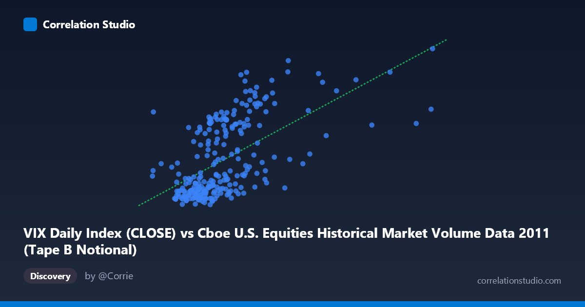
VIX Daily Index (CLOSE) vs Cboe U.S. Equities Historical Market Volume Data 2011 (Tape B Notional)

Pearson correlation (r): 0.5937
Spearman correlation: 0.6268
p-value: 0
Sample size (n): 252
95% confidence interval: 0.5074 to 0.6683
Granger causality: None
Granger optimal lag: 1

AI analysis

Scatterplot Analysis: VIX Daily Index vs. Tape B Notional Volume (2011)

Relationship Overview The scatterplot reveals a moderate positive relationship between the CBOE VIX Daily Index closing values and Tape B Notional trading volume across U.S. equities exchanges in 2011. As VIX levels rise — indicating higher market-implied volatility — Tape B Notional volume tends to increase as well. This is conceptually intuitive: periods of elevated fear or uncertainty in equity markets typically drive higher trading activity, as investors rebalance, hedge, or liquidate positions. The linear regression equation (y = 2.69e-9·x + 10.45) suggests a small but meaningful slope, where each unit increase in VIX corresponds to a measurable uptick in notional volume, though the relationship is far from deterministic.

Correlation Strength and Statistical Framing The Pearson correlation of r = 0.594 indicates a moderate positive association, but the more instructive figure is r² = 0.353: only about 35.3% of the variance in Tape B Notional volume is explained by VIX levels. This means nearly two-thirds of the variability in trading volume is driven by factors outside of VIX alone. The 95% confidence interval of [0.507, 0.668] is reasonably tight and lies entirely above zero, lending statistical credibility to the relationship. With a p-value effectively at zero across a paired sample of n = 252 (drawn from a population of N = 3,780), the correlation is highly unlikely to be a sampling artifact. However, the Granger causality results are notably null in both directions — VIX→Volume (F = 0.030, p = 0.864) and Volume→VIX (F < 0.001, p = 0.991) — meaning that despite the contemporaneous correlation, neither variable meaningfully predicts the other at a one-period lag. This is a critical caveat: correlation here appears to be contemporaneous co-movement, not a lead-lag predictive relationship.

Patterns, Clusters, and Outliers Several structural features stand out in the data. There appears to be a dense lower cluster where VIX values fall roughly between 14–22 and notional volume is relatively contained, suggesting a baseline "calm market" regime. Above a VIX threshold of approximately 25–30, the scatter begins to fan out considerably, hinting at heteroscedasticity — variance in notional volume increases as VIX rises. A handful of notable outliers are visible at the upper end: points with very high VIX readings (≥35–45) paired with exceptionally large notional volumes stand apart from the main cloud, likely corresponding to specific stress episodes in 2011 such as the U.S. debt ceiling crisis (August 2011) or the Eurozone sovereign debt turmoil, when VIX briefly spiked above 40 and trading surged. These extreme observations may be disproportionately driving the overall r value.

Confounding Factors and Caveats Several important caveats apply. First, 2011 was an atypical year — it included multiple tail-risk events that created episodic spikes in both VIX and volume, potentially inflating the apparent correlation beyond what would hold in calmer periods. Second, Tape B specifically covers NYSE MKT (AMEX) and regional exchanges, so its notional volume may reflect dynamics different from the broader market, introducing selection bias. Third, the absence of Granger causality signals that the co-movement is likely driven by a common latent factor — perhaps macroeconomic news shocks or systemic risk events — rather than a direct causal mechanism between these two variables. Finally, potential autocorrelation within the time series (daily observations over a full calendar year) may inflate confidence in the correlation estimate if standard independence assumptions are violated.

Actionable Insights and Further Investigation Practitioners should resist using VIX as a direct predictor of Tape B Notional volume at a one-day lag, given the flat Granger results. Instead, both variables should be treated as joint responses to underlying volatility regimes. A productive next step would be to segment the analysis by volatility regime (e.g., VIX < 20, 20–30, 30) to test whether the relationship strengthens nonlinearly in stress periods — the apparent heteroscedasticity strongly suggests this. Incorporating a regime-switching or threshold regression model could better capture the asymmetric dynamics visible in the scatter. Additionally, comparing Tape B results against Tape A and Tape C notional volumes would help assess whether this relationship is exchange-specific or market-wide. Finally, controlling for day-of-week effects, options expiration dates, and macro announcement days would help isolate whether the correlation persists after accounting for known volume drivers.

X dataset: Cboe U.S. Equities Historical Market Volume Data 2011

Y dataset: VIX Daily Index

Part of experiment: Daily - Cboe U.S. Equities Historical Market Volume Data 2011 vs VIX Daily Index