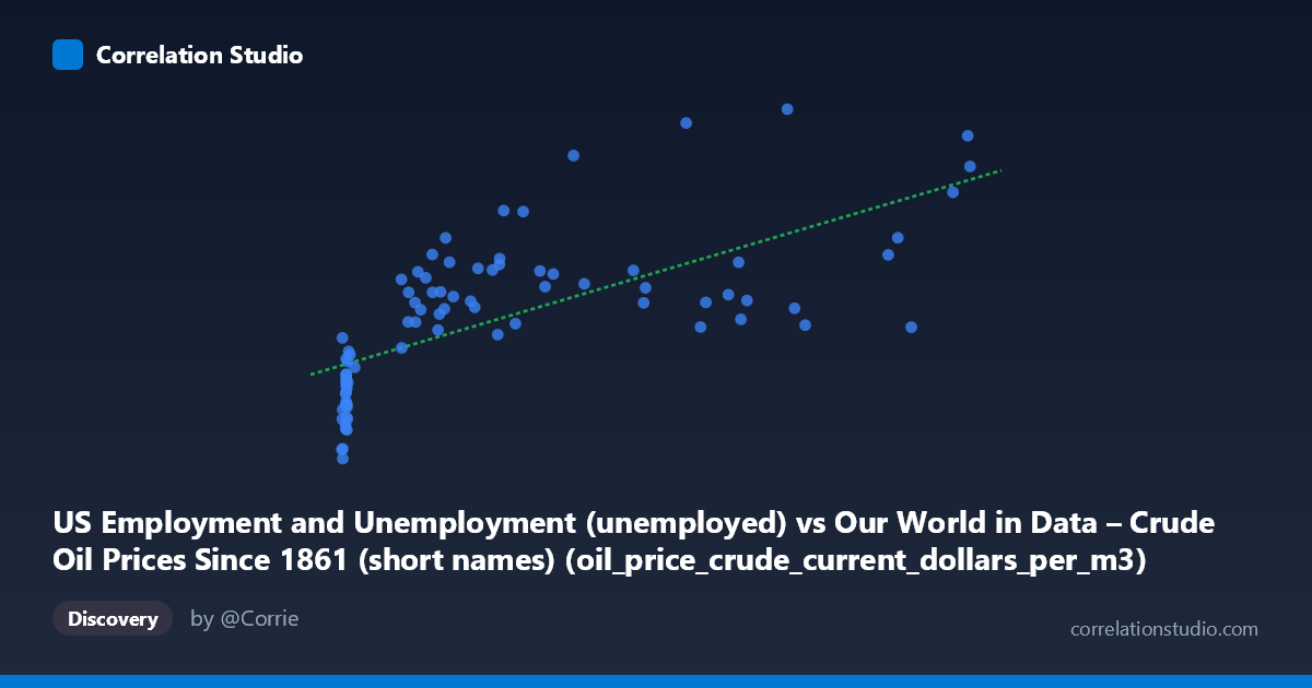
US Employment and Unemployment (unemployed) vs Our World in Data – Crude Oil Prices Since 1861 (short names) (oil_price_crude_current_dollars_per_m3)
- Pearson correlation (r)
- 0.6887
- Spearman correlation
- 0.8064
- p-value
- 0
- Sample size (n)
- 85
- 95% confidence interval
- 0.5574 to 0.7864
- Granger causality
- None
- Granger optimal lag
- 10
AI analysis
Analysis: US Unemployment vs. Crude Oil Prices (1941–2024)
1. What the Visualization Reveals
The scatterplot displays a positive but heteroscedastic relationship between the number of unemployed Americans (X-axis) and crude oil prices in current dollars per cubic meter (Y-axis) across roughly eight decades. At low unemployment values (roughly 6–20 units), oil prices scatter widely from near zero to mid-range values, while at higher unemployment figures the relationship appears to tighten somewhat around a rising trend. The linear regression line (y = 10.95x + 4375.63) captures a general upward slope, but the wide dispersion around it — particularly at the lower end of the unemployment range — immediately signals that a straight line is an imperfect summary of the data's structure.
2. Correlation Strength, Direction, and Causality
The Pearson r of 0.691 indicates a moderate-to-strong positive correlation, but the more telling statistic is r² = 0.478: only about 47.8% of the variance in oil prices is explained by unemployment levels, meaning more than half the variation is attributable to other forces entirely. The 95% confidence interval [0.560, 0.789] is reasonably tight and does not cross zero, and the p-value of 3.45×10⁻¹³ makes the correlation highly statistically significant — this is almost certainly not a chance finding given n = 84. However, the Granger causality results critically undercut any causal interpretation: neither direction (X→Y nor Y→X) reaches significance at the optimal 10-period lag (F = 0.91, p = 0.53 and F = 1.44, p = 0.19, respectively). This means that knowing past unemployment values does not improve predictions of future oil prices beyond chance, and vice versa — the correlation likely reflects a shared common driver rather than a direct predictive relationship between the two series.
3. Notable Patterns, Clusters, and Outliers
Several structural features stand out. There is a dense cluster of very low unemployment values (6–20 units) paired with a wide range of oil prices (670–5,560), corresponding to earlier decades when both unemployment counts and oil prices were historically low. A second, more dispersed cluster occupies the mid-range (80–350 unemployment units) with oil prices mostly between 5,000 and 10,000, reflecting the post-1970s era of oil price volatility. Several notable outliers demand attention: the point at approximately (500, 14,825) sits conspicuously above the regression line, likely reflecting the COVID-era oil price spike against pandemic-era unemployment; similarly, (387.90, 14,265) and (263.15, 12,947) appear elevated. Conversely, (637.28, 5,996) and (519.80, 6,080) fall well below the trend, suggesting periods of high unemployment without correspondingly high oil prices. The Spearman ρ exceeding Pearson r confirms that a logarithmic or power-law transformation of X would likely produce a better-fitting model, consistent with the visual impression that the relationship flattens somewhat at very high unemployment values.
4. Confounding Factors and Caveats
This correlation is a textbook candidate for spurious correlation driven by shared long-term trends. Both unemployment (as an absolute count rather than a rate) and nominal oil prices have grown substantially over 80+ years, driven by population growth, inflation, and economic expansion — they may simply be co-trending over time without meaningful mechanistic linkage. Using nominal oil prices (not inflation-adjusted) amplifies this problem, as dollar values naturally rise over decades regardless of real-world supply-demand dynamics. The unemployment figure appears to be an absolute count, which grows with the labor force even when the unemployment rate is stable. Additionally, oil prices are determined by global geopolitical events (OPEC embargoes, Gulf Wars, COVID demand collapse, Russia-Ukraine conflict) that operate largely independently of US labor market conditions. The 10-period optimal lag in the Granger test is unusually long (potentially 10 years in an annual series), which itself suggests the relationship is diffuse and temporally unstable rather than mechanistically direct.
5. Actionable Insights and Further Investigation
Several analytical steps would sharpen this investigation considerably. First, detrend both series (e.g., first-differencing or regressing out a time trend) to test whether the correlation survives removal of shared secular growth — this is the single most important diagnostic. Second, substitute real (inflation-adjusted) oil prices and the unemployment rate (rather than absolute count) to eliminate the most obvious spurious drivers. Third, fit a logarithmic regression of oil price on unemployment, given the Spearman Pearson signal, and compare AIC/BIC against the linear model. Fourth, introduce explicit time-period controls or conduct a rolling-window correlation to test whether the r = 0.69 relationship is stable across decades or driven by specific eras (e.g., post-2000 globalization, post-2008 financial crisis). Finally, consider multivariate modeling incorporating GDP growth, Federal Reserve interest rates, and global oil supply shocks as covariates — these are the more proximate drivers of both variables and would likely absorb most of the currently "explained" variance, potentially eliminating the apparent unemployment-oil price link entirely.
X dataset: Our World in Data – Crude Oil Prices Since 1861 (short names)
Y dataset: US Employment and Unemployment
Part of experiment: Yearly - Our World in Data – Crude Oil Prices Since 1861 (short names) vs US Employment and Unemployment