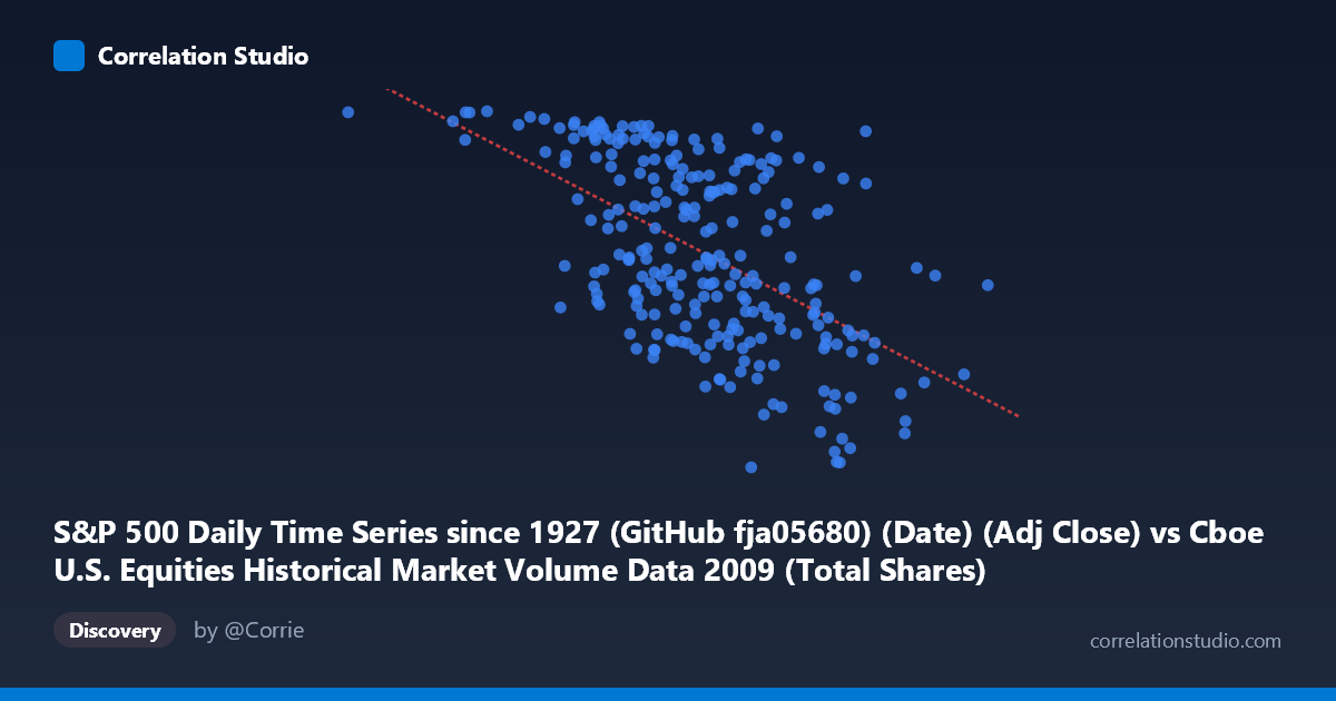
S&P 500 Daily Time Series since 1927 (GitHub fja05680) (Date) (Adj Close) vs Cboe U.S. Equities Historical Market Volume Data 2009 (Total Shares)

Pearson correlation (r): -0.5553
Spearman correlation: -0.5511
p-value: 0
Sample size (n): 252
95% confidence interval: -0.6353 to -0.4636
Granger causality: X → Y
Granger optimal lag: 10

AI analysis

Analysis: S&P 500 Price vs. U.S. Equity Market Trading Volume (2009)

Relationship Overview The scatterplot reveals a moderate negative relationship between S&P 500 adjusted closing prices (X-axis) and total U.S. equity market shares traded (Y-axis) across 2009. As S&P 500 prices increased throughout the year, aggregate trading volume tended to decline — a pattern consistent with the well-documented phenomenon of elevated trading activity during periods of market stress and uncertainty. The linear regression equation (y = -4.13×10⁻⁷x + 1261.75) captures this inverse trend, suggesting that for every ~2.4 million point increase in the index level, total shares traded declined by roughly one unit on the Y-scale. Given that 2009 spanned the tail end of the financial crisis and a dramatic recovery rally, this inverse dynamic reflects a behaviorally intuitive story: panic-driven volume gives way to calmer, lower-volume appreciation.

Correlation Strength and Statistical Significance The Pearson correlation of r = -0.5553 indicates a moderate negative association, but the more interpretively honest metric is r² = 0.3084 — meaning S&P 500 price levels explain only about 30.8% of the variance in daily trading volume. Nearly 70% of volume variability is driven by factors not captured here. The 95% confidence interval of [-0.6353, -0.4636] is reasonably tight and excludes zero, and the p-value of effectively 0 (against N = 3,232) confirms this is not a chance finding. Crucially, the Granger causality analysis supports a unidirectional temporal relationship: X Granger-causes Y (F = 2.384, p = 0.0106) at a 10-period lag, while the reverse direction fails to reach significance (p = 0.081). This means S&P 500 price movements have statistically meaningful predictive power over subsequent trading volume roughly two weeks out, but volume does not reliably predict future price — an asymmetry with practical trading implications.

Patterns, Clusters, and Outliers Several structural features stand out in the data. There is a visible high-volume, low-price cluster concentrated in the X range of roughly 192M–600M (early 2009, near market lows), where Y values frequently exceed 1,050–1,127 shares — consistent with crisis-era panic selling and forced liquidations. Conversely, a low-volume, moderate-to-high price cluster appears in the 900M–1,200M range, reflecting the post-March 2009 recovery rally. The point at (192,269,942.50, 1126.48) is a notable outlier representing an extreme volume day near the market bottom. Similarly, (1,212,524,830.85, 907.39) anchors the upper price extreme with relatively subdued volume. Some scatter in the mid-range (700M–900M) suggests the relationship is not strictly linear, with considerable dispersion — hinting at regime-dependent behavior or episodic volume spikes unrelated to price level.

Confounding Factors and Caveats Several important caveats temper interpretation. First, 2009 is a highly unusual year — a once-in-a-generation market collapse followed by a 60%+ rally — making any correlation derived from it potentially non-generalizable. The inverse relationship may be largely an artifact of this specific crisis-recovery trajectory rather than a structural feature. Second, trading volume is influenced by many factors independent of price: option expiration cycles, index rebalancing, institutional program trading, ETF creation/redemption, and regulatory changes (e.g., uptick rule elimination effects). Third, the axes encode time implicitly (X-axis values proxy for calendar progression as the market rose), meaning some of the observed correlation may reflect a shared time trend rather than a true causal mechanism. Fourth, the Granger causality result, while statistically significant, explains modest incremental variance and should not be conflated with economic causation.

Actionable Insights and Further Investigation Practitioners could use the 10-period Granger lag as a starting signal in volume-forecasting models — rising price momentum may serve as a weak but statistically valid leading indicator of declining volume ~2 weeks ahead, useful for liquidity and execution planning. More rigorously, this analysis warrants decomposing both series to remove the shared time trend before re-estimating correlation, which would clarify whether the relationship persists beyond the 2009 calendar effect. Extending the dataset to multiple years would test whether this inverse relationship holds in non-crisis periods or reverses in bull markets. Additionally, segmenting by market regime (e.g., high-VIX vs. low-VIX periods) could reveal whether the negative correlation is concentrated in stress episodes — a finding that would have direct implications for volatility-adjusted trading strategies.

X dataset: Cboe U.S. Equities Historical Market Volume Data 2009

Y dataset: S&P 500 Daily Time Series since 1927 (GitHub fja05680) (Date)

Part of experiment: Daily - Cboe U.S. Equities Historical Market Volume Data 2009 vs S&P 500 Daily Time Series since 1927 (GitHub fja05680) (Date)