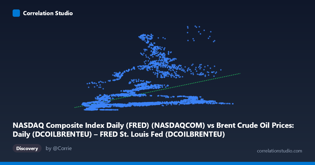
NASDAQ Composite Index Daily (FRED) (NASDAQCOM) vs Brent Crude Oil Prices: Daily (DCOILBRENTEU) – FRED St. Louis Fed (DCOILBRENTEU)
- Pearson correlation (r)
- 0.4518
- Spearman correlation
- 0.7084
- p-value
- 0
- Sample size (n)
- 9718
- 95% confidence interval
- 0.4358 to 0.4675
- Granger causality
- None
- Granger optimal lag
- 9
AI analysis
NASDAQ Composite vs. Brent Crude Oil: Correlation Analysis
1. Overall Relationship Revealed
The scatterplot reveals a weakly positive but highly dispersed relationship between the NASDAQ Composite Index and Brent Crude Oil prices. While a upward-trending regression line (y = 71.77x + 878.25) is present, the data cloud is extraordinarily wide, with Y-values (NASDAQ) ranging from under 300 to over 26,000 for similar X-values (Brent crude). This visual scatter immediately signals that crude oil price is a poor standalone predictor of NASDAQ performance. The relationship, while statistically detectable across nearly 10,000 paired observations spanning 1987–2026, is practically tenuous at best.
2. Correlation Strength, Direction, and Causality
The Pearson r of 0.4518 indicates a moderate positive correlation, but the explanatory power is modest: R² = 0.204, meaning Brent crude prices account for only ~20% of the variance in the NASDAQ Index. The remaining ~80% of NASDAQ variability is driven by factors entirely unrelated to oil prices. The 95% confidence interval [0.4358, 0.4675] is narrow — a consequence of the large sample (n = 9,718) — confirming the correlation estimate is precise, but precision should not be conflated with practical significance. The p-value of effectively zero confirms this is not a chance finding, but statistical significance here is largely a function of enormous sample size rather than a strong underlying signal.
Critically, the Granger causality tests find no significant predictive direction in either direction (X→Y: F = 0.919, p = 0.508; Y→X: F = 1.367, p = 0.197). Even at an optimal lag of 9 periods, neither variable reliably predicts the other temporally. This is an important finding: the correlation, whatever its origin, does not reflect a forecasting relationship. One cannot use today's Brent price to predict tomorrow's NASDAQ movement, nor vice versa.
3. Notable Patterns, Clusters, and Outliers
Several structural features stand out in the sample points:
- Low-X cluster (Brent < ~30 USD/barrel): Predominantly associated with early data (pre-2000s), where NASDAQ values were also low, creating a dense cluster in the lower-left — this likely reflects the pre-dot-com era rather than a causal link. - High-Y outliers: Points like (72.06, 20,585), (81.72, 14,226), and (72.44, 15,115) show extreme NASDAQ values at moderate oil prices, representing the post-2010 NASDAQ tech boom era when oil was range-bound while equities surged. - High-X, moderate-Y points: Observations like (134.43, 2,459) and (108.84, 3,020) show very high crude prices with relatively low NASDAQ values, consistent with the 2008 oil spike period when equities were under stress — a negative relationship in that regime. - The Spearman ρ exceeding Pearson r confirms a non-linear structure in the data. A logarithmic or polynomial fit would likely capture the relationship more accurately than the linear regression applied here.
4. Confounding Factors and Caveats
This correlation almost certainly reflects shared temporal trends rather than a direct economic mechanism. Both series trend upward over the 1987–2026 window due to inflation, economic growth, and dollar dynamics — a classic spurious correlation via common time trend. Key confounders include:
- Macroeconomic cycles: Recessions (2001, 2008, 2020) simultaneously suppress oil demand and equity prices, inducing positive correlation without causation. - Dollar strength: A weaker USD inflates both oil prices (dollar-denominated commodity) and boosts multinational earnings reflected in NASDAQ. - Regime shifts: The relationship likely reverses sign in oil-shock regimes (e.g., 1990, 2008), where high oil prices act as a tax on economic activity and harm tech equities — this regime heterogeneity is masked by the aggregate correlation. - The axes appear to be swapped from convention (NASDAQ on X, Brent on Y based on axis labels vs. dataset descriptions) — analysts should verify variable assignment before acting on the regression coefficients.
5. Actionable Insights and Further Investigation
- Detrend both series (e.g., first differences or log-returns) before recalculating correlation; the raw-level correlation is almost certainly inflated by shared upward trends. Returns-based correlation would be far more actionable for trading or hedging purposes. - Fit a non-linear model (logarithmic or piecewise) given the Spearman Pearson signal; the linear R² of 20.4% likely understates fit in some regimes and overstates it in others. - Segment by macroeconomic regime (expansion vs. recession, low vs. high volatility) to test whether the correlation changes sign or magnitude — this would reveal whether any hedging relationship exists conditionally. - Investigate sector-level NASDAQ components (energy vs. tech vs. biotech) separately; energy stocks within NASDAQ may show a very different relationship to Brent than the composite index overall. - Given the absence of Granger causality, this relationship should not be used for short-term forecasting models in either direction without substantially richer conditioning variables.
X dataset: Brent Crude Oil Prices: Daily (DCOILBRENTEU) – FRED St. Louis Fed
Y dataset: NASDAQ Composite Index Daily (FRED)
Part of experiment: Daily - Brent Crude Oil Prices: Daily (DCOILBRENTEU) – FRED St. Louis Fed vs NASDAQ Composite Index Daily (FRED)