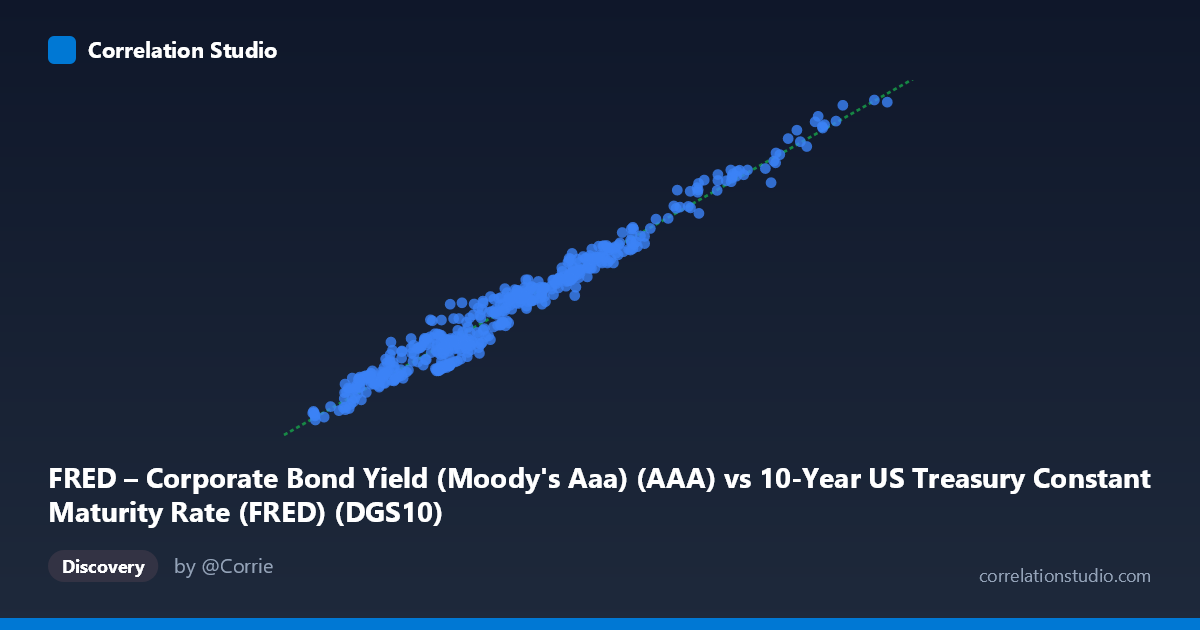
FRED – Corporate Bond Yield (Moody's Aaa) (AAA) vs 10-Year US Treasury Constant Maturity Rate (FRED) (DGS10)
- Pearson correlation (r)
- 0.9842
- Spearman correlation
- 0.9739
- p-value
- 0
- Sample size (n)
- 492
- 95% confidence interval
- 0.9812 to 0.9867
- Granger causality
- None
- Granger optimal lag
- 1
AI analysis
Analysis: Corporate Bond Yield vs. 10-Year Treasury Rate
1. Overall Relationship The scatterplot reveals a strikingly tight, positive linear relationship between Moody's Aaa corporate bond yields and the 10-Year US Treasury constant maturity rate. The data points cluster closely around the regression line (y = 0.897x + 1.637), forming a near-perfect diagonal band from the lower-left to the upper-right of the chart. This pattern is consistent with well-established fixed-income theory: corporate bond yields and Treasury yields are driven by the same macroeconomic forces — inflation expectations, Federal Reserve policy, and broader economic growth outlook — making their co-movement both expected and intuitive.
2. Correlation Strength and Statistical Framing With r = 0.9842, this is one of the strongest real-world financial correlations observable. The r² of 0.9687 means that approximately 96.9% of the variance in Treasury yields is explained by Aaa corporate bond yields (or vice versa), leaving only ~3.1% attributable to other factors. The 95% confidence interval of [0.9812, 0.9867] is exceptionally narrow, confirming that this result is highly stable and not driven by sampling artifact — and with a p-value of effectively zero across 492 paired observations, there is no plausible statistical uncertainty about the existence of this relationship. The regression slope of ~0.897 is slightly below 1.0, indicating that corporate yields move nearly in lockstep with Treasuries, but with a modest dampening effect, while the intercept of ~1.637 reflects the persistent credit spread — the yield premium investors demand for holding corporate rather than government debt. Notably, the Granger causality tests find no significant directional predictive relationship in either direction (X→Y: F=0.031, p=0.860; Y→X: F=0.039, p=0.844), meaning that knowing today's corporate yield does not help predict tomorrow's Treasury yield beyond what is already known, and vice versa. This strongly suggests both series are driven by common underlying forces rather than one leading the other.
3. Patterns, Clusters, and Outliers The sample points reveal several notable features. The data naturally clusters into at least two broad regimes: a low-rate cluster (X roughly 1–5%, Y roughly 2–6%) corresponding to the post-2008 and post-2020 era of unconventional monetary policy, and a high-rate cluster (X roughly 7–15%, Y roughly 8–16%) corresponding to the inflationary 1970s–1980s. The point at approximately (14.05, 14.32) and (13.63, 13.55) represent the extreme high-rate environment of the early 1980s Volcker era, sitting at the far upper-right of the chart — they are not statistical outliers in the sense of deviating from the trend, but they are leverage points that anchor the regression. At the lower end, points like (1.31, 2.53) reflect the post-COVID zero-rate environment. The spread between X and Y (the credit spread) appears to widen slightly at lower rate levels, consistent with the non-zero intercept — when Treasury rates are very low, the absolute credit spread becomes more visible as a proportion of yield.
4. Confounding Factors and Caveats Several important caveats apply. First, this is a spurious-correlation-resistant but not causation-proof relationship — both series share common drivers (inflation, Fed policy, economic cycles), so the high r² reflects a shared response to macro conditions rather than a direct causal mechanism, as confirmed by the Granger results. Second, the time span of 64 years (1962–2026) encompasses dramatically different monetary regimes, and pooling these together can mask structural breaks; a single regression line may misrepresent behavior within any specific sub-period. Third, the credit spread (the intercept) is not constant — it compresses during risk-on periods and widens during financial stress (e.g., 2008–2009), meaning residuals from this regression would be economically meaningful and not simply noise. Fourth, with monthly or lower-frequency aggregation at lag-1, the Granger test may lack the temporal resolution to detect any short-run lead-lag dynamics present in daily data.
5. Actionable Insights and Further Investigation Several analytical extensions would add significant value. Regime-segmented analysis — splitting the data into pre- and post-1990, or by Fed policy cycle — would reveal whether the slope and intercept have shifted structurally over time. Modeling the residuals (credit spread) as a separate time series is arguably more interesting than the raw correlation: the spread is where economic signal lives, capturing risk appetite, default expectations, and liquidity conditions. Analysts could investigate whether the spread Granger-causes equity volatility or recession indicators, which the raw yield correlation cannot reveal. Additionally, testing this relationship at daily frequency with shorter lags might uncover transient lead-lag dynamics invisible at the monthly level. Finally, incorporating a third variable such as the VIX, inflation breakevens, or Fed Funds rate would help determine what portion of the unexplained 3.1% variance is systematic versus idiosyncratic — potentially yielding a more complete fixed-income yield model.
X dataset: 10-Year US Treasury Constant Maturity Rate (FRED)
Y dataset: FRED – Corporate Bond Yield (Moody's Aaa)
Part of experiment: Daily - 10-Year US Treasury Constant Maturity Rate (FRED) vs FRED – Corporate Bond Yield (Moody's Aaa)