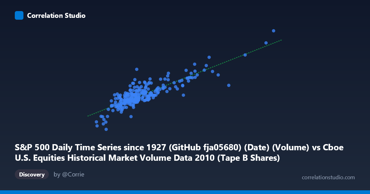
S&P 500 Daily Time Series since 1927 (GitHub fja05680) (Date) (Volume) vs Cboe U.S. Equities Historical Market Volume Data 2010 (Tape B Shares)
- Pearson correlation (r)
- 0.8518
- Spearman correlation
- 0.7703
- p-value
- 0
- Sample size (n)
- 252
- 95% confidence interval
- 0.8139 to 0.8825
- Granger causality
- None
- Granger optimal lag
- 10
AI analysis
Scatterplot Analysis: S&P 500 Volume vs. Cboe Tape B Shares (2010)
Relationship Overview The scatterplot reveals a strong positive linear relationship between total U.S. equities market volume (X-axis, measured by S&P 500 daily volume as a proxy) and Cboe Tape B share volume (Y-axis) across 252 trading days in 2010. As overall market volume rises, Tape B share volume increases correspondingly, which is intuitive — Tape B covers NYSE American-listed securities, and its trading activity broadly tracks the rhythm of the wider equity market. The linear regression equation (y = 22.63x + ~2.01B) confirms a consistent proportional scaling relationship throughout the year.
Correlation Strength and Statistical Significance The Pearson correlation of r = 0.852 is statistically robust, and the r² = 0.726 indicates that approximately 72.6% of the daily variance in Tape B share volume is explained by overall market volume — a substantial explanatory share, though ~27% remains attributable to other factors. The 95% confidence interval of [0.814, 0.883] is narrow and entirely in positive territory, reinforcing high statistical confidence in this relationship. With a p-value effectively at zero across a paired sample of 252 observations drawn from a population of 3,302, the correlation is unambiguously significant. However, Granger causality tests tell a more cautious story: neither direction (X→Y nor Y→X) reaches significance at the optimal 10-period lag (F = 1.15, p = 0.33 and F = 0.27, p = 0.99, respectively). This means that while the two series move together, neither reliably predicts the other in a temporal sense — the relationship is contemporaneous co-movement, not directional causation.
Notable Patterns, Clusters, and Outliers The bulk of observations form a relatively tight, well-behaved linear cluster concentrated in the ranges of ~70M–150M for X and ~3.1B–6.2B for Y, consistent with the mean values. Several notable outliers deserve attention: - A high-leverage point near (316M, 9.47B) sits far to the upper right and appears to exert significant influence on the regression slope — this likely corresponds to an unusually high-volume trading day (possibly tied to a macro event, options expiration, or index rebalancing). - A point near (255M, 5.45B) is anomalous in a different way — very high X volume but comparatively modest Y volume, suggesting Tape B did not proportionally participate in that market-wide surge, perhaps indicating the volume spike was concentrated in large-cap NYSE or Nasdaq names outside Tape B coverage. - A point near (53M, 1.29B) anchors the lower left as the minimum, possibly a holiday-shortened session.
Confounding Factors and Caveats Several important caveats apply. First, the X-axis variable is labeled as S&P 500 volume but is being used as a proxy for total U.S. market volume — these are not equivalent, and the S&P 500 skews heavily toward large-cap NYSE/Nasdaq securities, which may not mirror Tape B dynamics uniformly. Second, both series likely share a strong common driver: overall market liquidity conditions, macroeconomic sentiment, and calendar effects (e.g., quarter-end, expiration Fridays) simultaneously inflate or deflate both measures, making correlation partially spurious by shared external forcing. Third, the absence of Granger causality is a critical reminder that high correlation in daily financial data often reflects common responses to news or structural market conditions rather than any mechanistic linkage. Finally, 2010 was a single, somewhat unusual post-financial-crisis recovery year, limiting generalizability.
Actionable Insights and Further Investigation The strong contemporaneous correlation makes Tape B volume reasonably predictable from broad market volume on the same day, which could be useful for liquidity estimation or market microstructure modeling intraday. However, given the Granger non-causality, practitioners should not use lagged overall volume to forecast next-period Tape B volume — the predictive window is same-day only. Further investigation should examine: (1) whether the outlier near (316M, 9.47B) corresponds to a specific identifiable event and whether removing it materially changes regression coefficients; (2) extending the analysis across multiple years to test whether the 2010 relationship is stable or regime-dependent; (3) decomposing the unexplained 27% variance by introducing additional predictors such as VIX, sector rotation signals, or intraday volume profiles; and (4) testing whether a non-linear or piecewise model better handles the apparent heteroscedasticity visible at higher volume levels.
X dataset: Cboe U.S. Equities Historical Market Volume Data 2010
Y dataset: S&P 500 Daily Time Series since 1927 (GitHub fja05680) (Date)
Part of experiment: Daily - Cboe U.S. Equities Historical Market Volume Data 2010 vs S&P 500 Daily Time Series since 1927 (GitHub fja05680) (Date)