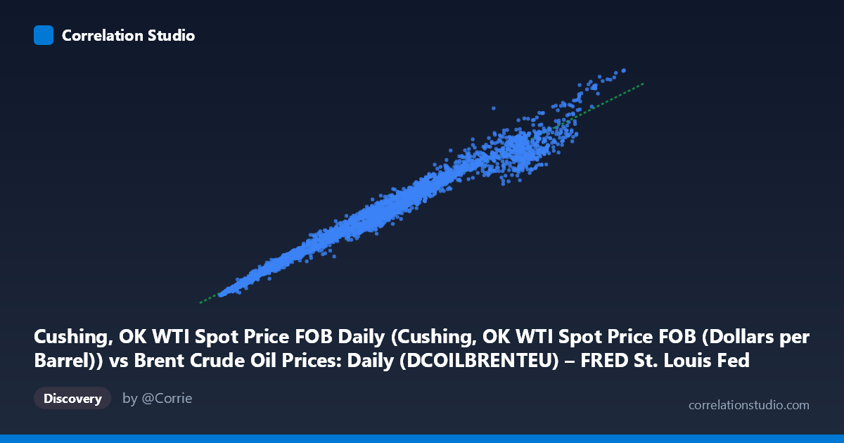
Cushing, OK WTI Spot Price FOB Daily (Cushing, OK WTI Spot Price FOB (Dollars per Barrel)) vs Brent Crude Oil Prices: Daily (DCOILBRENTEU) – FRED St. Louis Fed (DCOILBRENTEU)
- Pearson correlation (r)
- 0.9911
- Spearman correlation
- 0.995
- p-value
- 0
- Sample size (n)
- 9718
- 95% confidence interval
- 0.9907 to 0.9914
- Granger causality
- None
- Granger optimal lag
- 1
AI analysis
WTI vs. Brent Crude Oil Price Correlation Analysis
Relationship Overview
The scatterplot reveals an exceptionally tight, near-linear positive relationship between WTI (West Texas Intermediate) and Brent crude oil spot prices across nearly four decades of daily observations (1987–2026). The data points form a dense, narrow band along the regression line (y = 0.886x + 4.13), indicating that the two benchmarks move in near-perfect lockstep across a wide price range — from roughly $10/barrel up to approximately $145/barrel. This is consistent with what energy economists would expect: both are global crude oil benchmarks responding to the same fundamental supply-demand dynamics, geopolitical events, and macroeconomic cycles.
Correlation Strength and Statistical Significance
The correlation is extraordinarily strong (r = 0.9911), with R² = 0.9823 meaning 98.2% of the daily variance in Brent prices is explained by WTI prices, leaving only ~1.8% attributable to other factors. The 95% confidence interval [0.9907, 0.9914] is vanishingly narrow given the large sample (n = 9,718 paired observations), and the p-value of effectively zero confirms this is not a chance finding. However, the Granger causality results are notably telling: neither direction (X→Y nor Y→X) achieves statistical significance at lag-1 (WTI→Brent: F = 1.06, p = 0.303; Brent→WTI: F = 0.94, p = 0.332). This means that, despite the overwhelming contemporaneous correlation, neither price series reliably predicts the other one period ahead — they are better understood as simultaneously driven by shared global factors rather than one leading the other in any exploitable temporal sense.
Notable Patterns, Clusters, and Structural Features
Several structural features stand out in the sample points and implied scatter. There is a notable cluster of observations in the $10–$30/barrel range, reflecting the prolonged low-price environment of the late 1980s through mid-1990s, and another dense cluster around $15–$25 visible in the sample data. A second, more dispersed cluster appears in the $60–$115 range, corresponding to the 2000s commodity supercycle and post-2010 era. The regression slope of 0.886 (less than 1.0) is structurally important: it means Brent systematically trades at a premium to WTI, especially at higher price levels — a real-world phenomenon known as the WTI-Brent spread, driven by U.S. pipeline infrastructure constraints, landlocked delivery at Cushing, Oklahoma, and differing regional supply-demand balances. Points like (135.81, 141.47) and (110.37, 103.46) confirm this divergence widens at extremes.
Confounding Factors and Interpretive Caveats
While the correlation is statistically overwhelming, several caveats merit attention. First, the WTI-Brent spread is not constant — it collapsed during periods of U.S. export restrictions and widened dramatically during 2011–2014 when Cushing pipeline bottlenecks caused WTI to trade at an unusual discount to Brent; this structural break may not be fully visible in aggregate statistics but would create heteroscedasticity in residuals. Second, the axes appear swapped in the dataset labeling (WTI is on the X-axis but described under the Brent dataset header, and vice versa) — analysts should verify column assignments before drawing directional conclusions. Third, daily price data exhibits strong autocorrelation, which inflates the effective sample size and can make already-significant p-values appear even more extreme, though the Granger test appropriately accounts for this. Finally, both series are non-stationary (prices follow near-random-walk behavior), meaning the correlation, while real, partly reflects shared trending rather than a stable structural equation.
Actionable Insights and Further Investigation
Several avenues warrant deeper investigation. Spread analysis — modeling the WTI-Brent differential directly as a time series — would be more actionable for traders and refiners than the raw correlation, particularly identifying regime changes (pre/post-2011 U.S. export ban repeal). Analysts should apply cointegration testing (e.g., Engle-Granger or Johansen) rather than simple correlation, as cointegration would confirm whether the spread is mean-reverting and thus tradeable. The residuals from the linear regression should be examined for clustering by year to detect structural breaks. For forecasting applications, a Vector Error Correction Model (VECM) would better capture the long-run equilibrium relationship and short-run deviations than either Granger test or OLS alone. Finally, incorporating confounding covariates — USD index, global inventory levels, OPEC production decisions, and U.S. crude export volumes — would help explain the residual 1.8% variance and provide a more complete causal model of global crude oil price formation.
X dataset: Brent Crude Oil Prices: Daily (DCOILBRENTEU) – FRED St. Louis Fed
Y dataset: Cushing, OK WTI Spot Price FOB Daily
Part of experiment: Daily - Brent Crude Oil Prices: Daily (DCOILBRENTEU) – FRED St. Louis Fed vs Cushing, OK WTI Spot Price FOB Daily