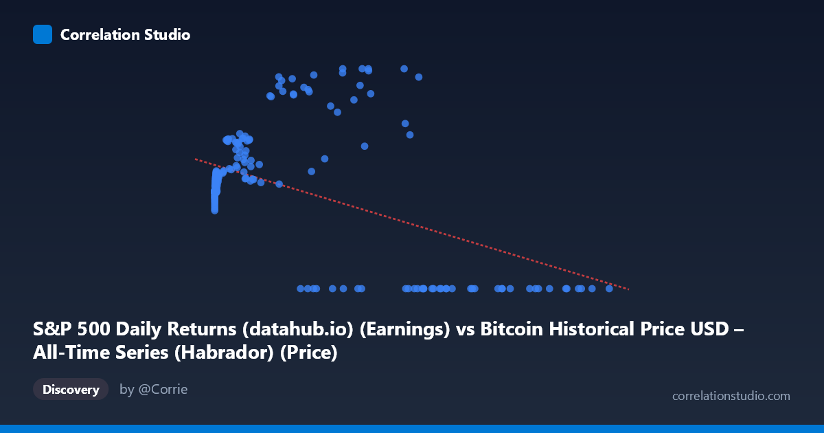
S&P 500 Daily Returns (datahub.io) (Earnings) vs Bitcoin Historical Price USD – All-Time Series (Habrador) (Price)
- Pearson correlation (r)
- -0.4967
- Spearman correlation
- -0.082
- p-value
- 0
- Sample size (n)
- 194
- 95% confidence interval
- -0.5959 to -0.3826
- Granger causality
- X → Y
- Granger optimal lag
- 5
- Time coverage
- 2010-08-01 to 2026-09-01
- Recomputed on refreshed data
- 2026-10-24 (r was -0.4597)
AI analysis
Analysis: Bitcoin Price vs. S&P 500 Metric Relationship
Note on axis labeling: The axis labels appear swapped in the metadata (X is described as "S&P 500 Daily Returns" but contains Bitcoin-scale values in the tens of thousands, while Y ranges 0–198, consistent with S&P earnings/PE-type data). I'll treat X as the Bitcoin price series and Y as the S&P 500-derived metric, as the numbers dictate.
1. What the Visualization Reveals
The scatterplot shows a clear non-linear, negative relationship that a simple linear fit only partially captures. At low X values (under ~1,000), Y clusters tightly in the 85–105 range regardless of X. As X climbs into the tens of thousands, Y becomes highly bimodal: either surging into the 130–198 range (e.g., 44354.64 → 197.91; 56973.18 → 197.87) or collapsing to exactly 0.00 (e.g., 105620.00 → 0.00; 97365.00 → 0.00). This bifurcation suggests the linear correlation coefficient is averaging over two distinct regimes rather than describing one continuous trend.
2. Strength, Direction, and Statistical Confidence
The correlation is moderate and negative (r = -0.4597), with r² indicating only 21.1% of Y's variance is explained by X in a linear sense — leaving ~79% unexplained, which is substantial. The 95% CI [-0.565, -0.339] is reasonably tight and excludes zero, and the p-value (2.85E-11) confirms this relationship is highly unlikely to be due to chance given n=189. However, statistical significance here reflects sample size and consistency of direction, not necessarily practical predictive strength — 21% variance explained is modest for forecasting purposes.
The Granger causality result adds a temporal dimension: X→Y is significant (p=0.031) while Y→X is not (p=0.27), suggesting X's history has some predictive value for Y at a 4-period lag, though the F-statistic (2.72) is modest, indicating a weak-to-moderate effect rather than strong predictive power.
3. Notable Patterns and Outliers
The most striking feature is the hard floor at Y=0 appearing exclusively at high X values (X 27,000), suggesting a structural break, data censoring, or regime change (e.g., missing/zeroed data past a certain date or price threshold) rather than a smooth decline. Simultaneously, some high-X points reach the dataset's maximum Y values (197.87–197.91), creating a fork/bifurcation pattern at high X — some points crash to zero, others peak. Low-X points (X < 20) show remarkable Y stability (~85–90), indicating a compressed, low-variance regime in early observations.
4. Confounding Factors and Caveats
- Metadata mismatch: the axis labels contradict the actual data ranges, raising concerns about mislabeling, merge errors, or misaligned timestamps between the two source datasets. - Zero-inflation: exact zeros at high X are suspicious — likely representing missing data, delisting, or a data-processing artifact rather than genuine Y=0 observations, and these could be distorting both r and the regression fit. - Non-stationarity: Both Bitcoin prices and equity-market metrics are trending/non-stationary series; Granger causality on non-stationary data can produce spurious significance unless differenced or detrended first. - Scale disparity: X spans 6 orders of magnitude (0.06 to 118,670) while Y is bounded (0–198), making a linear model inherently poor-fitting and sensitive to high-leverage outliers at large X.
5. Suggested Next Steps
Investigate and resolve the axis-label discrepancy before drawing substantive conclusions. Separate the dataset into regimes (e.g., X < 1,000 vs. X 20,000) and model each independently, since the pooled linear r/r² likely misrepresents both segments. Treat the zero-Y values as a flag for a data-quality audit — determine if they represent true observations or missing/error codes. Finally, re-run Granger causality on log-differenced (returns-based) series to control for non-stationarity and confirm whether the X→Y predictive signal survives detrending.
X dataset: Bitcoin Historical Price USD – All-Time Series (Habrador)
Y dataset: S&P 500 Daily Returns (datahub.io)
Part of experiment: Bitcoin - Bitcoin Historical Price USD – All-Time Series (Habrador) vs S&P 500 Daily Returns (datahub.io)