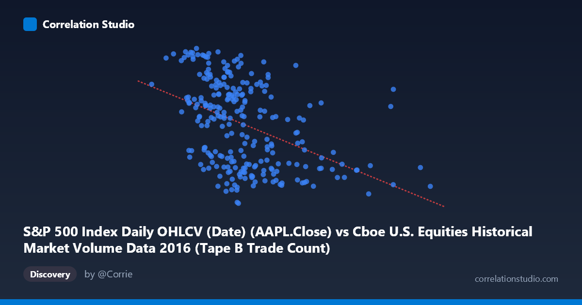
S&P 500 Index Daily OHLCV (Date) (AAPL.Close) vs Cboe U.S. Equities Historical Market Volume Data 2016 (Tape B Trade Count)

Pearson correlation (r): -0.4345
Spearman correlation: -0.4645
p-value: 0
Sample size (n): 252
95% confidence interval: -0.5297 to -0.3286
Granger causality: None
Granger optimal lag: 1

AI analysis

Scatterplot Analysis: AAPL Close Price vs. Cboe Tape B Trade Count (2016)

Relationship Overview The scatterplot reveals a moderate negative relationship between Apple's daily closing price (S&P 500 dataset) and the Cboe U.S. Equities Tape B Trade Count throughout 2016. As AAPL's closing price increased, Tape B trade counts tended to decline. The linear regression equation (y = -3.50097E-05x + 115.783) confirms this inverse slope, suggesting that for every ~28,600-point increase in AAPL's closing price (in the units represented on the X-axis, likely scaled), the Tape B trade count decreases by approximately 1 unit. Visually, the data cloud tilts downward from left to right, though with considerable scatter around the trend line.

Correlation Strength and Statistical Significance The Pearson correlation of r = -0.4345 indicates a moderate negative association, but the explanatory power is limited — r² = 0.1888 means only ~18.9% of the variance in Tape B Trade Count is explained by AAPL's closing price, leaving over 81% attributable to other factors. The 95% confidence interval of [-0.5297, -0.3286] is entirely negative and does not cross zero, lending credibility to the direction of the effect. The p-value of 4.978E-13 is extraordinarily small, confirming this correlation is highly unlikely to be a chance result given n = 252 paired observations. However, statistical significance should not be conflated with practical significance — the modest r² tempers enthusiasm for treating this as a strong predictive relationship. Critically, Granger causality tests show no significant directional predictability in either direction (X→Y: F = 0.64, p = 0.42; Y→X: F = 0.51, p = 0.48), meaning neither variable reliably predicts the other's future values at a one-period lag. This strongly suggests the observed correlation reflects a shared temporal trend or common external driver rather than any causal mechanism.

Notable Patterns, Clusters, and Outliers The bulk of the data clusters between roughly X = 200,000–400,000 and Y = 90–118, forming a moderately dense central band. Several high-X outliers are visible in the 450,000–715,000 range (notably one point near 558,000), consistently associated with lower Tape B trade counts (Y ≈ 93–97), which amplifies the negative slope. There also appears to be a bifurcated vertical spread within the central X range — at similar AAPL price levels, trade counts span nearly the full Y range (90–118), indicating substantial day-to-day variability in market activity that price alone cannot explain. No strong non-linear (e.g., U-shaped or exponential) pattern is apparent, suggesting the linear model is a reasonable but incomplete descriptor.

Confounding Factors and Caveats Several important caveats apply. First, AAPL's closing price follows a temporal trajectory — it trended upward through much of 2016 — while Tape B trade counts may have trended in the opposite direction due to secular market microstructure shifts (e.g., declining retail participation, venue fragmentation). This creates a spurious time-trend correlation that does not imply any economic link between the two. Second, Tape B covers NYSE American-listed securities, which are largely independent of AAPL (a Nasdaq/Tape C stock), making a direct causal story implausible on its face. Third, macroeconomic events in 2016 (Brexit, U.S. election volatility) could simultaneously affect both series in ways that inflate or distort the correlation. The Granger causality null results reinforce that this is likely a coincidental co-movement rather than a meaningful relationship.

Actionable Insights and Further Investigation Given the absence of Granger causality and low r², this correlation should not be used for predictive modeling in its current form. Recommended next steps include: (1) detrending both series (e.g., using first differences or residuals from a time trend) to test whether the correlation persists after removing shared temporal drift; (2) introducing control variables such as overall market volatility (VIX), total U.S. equity volume, or macroeconomic indicators to assess whether the relationship is spurious; (3) extending the lag structure in Granger tests beyond 1 period to check for delayed predictive effects; and (4) segmenting the data by market regime (pre/post-election, high/low volatility periods) to determine whether the negative correlation is driven by specific episodes rather than a stable structural relationship. These steps would clarify whether any operationally useful signal exists within this dataset pairing.

X dataset: Cboe U.S. Equities Historical Market Volume Data 2016

Y dataset: S&P 500 Index Daily OHLCV (Date)

Part of experiment: Daily - Cboe U.S. Equities Historical Market Volume Data 2016 vs S&P 500 Index Daily OHLCV (Date)