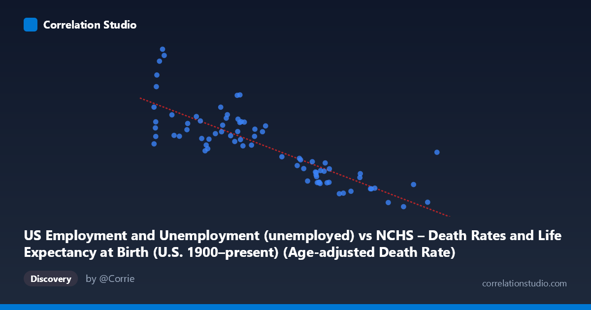
US Employment and Unemployment (unemployed) vs NCHS – Death Rates and Life Expectancy at Birth (U.S. 1900–present) (Age-adjusted Death Rate)
- Pearson correlation (r)
- -0.8256
- Spearman correlation
- -0.8323
- p-value
- 0
- Sample size (n)
- 78
- 95% confidence interval
- -0.8855 to -0.7388
- Granger causality
- None
- Granger optimal lag
- 10
- Time coverage
- 1941-01-01 to 2018-01-01
AI analysis
Analysis: U.S. Unemployment vs. Age-Adjusted Death Rate (1941–2018)
Relationship Overview
The scatterplot reveals a strong negative association between the number of unemployed Americans and the age-adjusted death rate: as unemployment figures rise, death rates tend to be lower, and as unemployment falls, death rates tend to be higher. The linear regression equation (y = −9.25x + 17,136.9) captures this inverse slope, predicting roughly a 9.25-unit decline in the death rate for each additional thousand unemployed workers. At first glance this relationship appears counterintuitive — higher unemployment is typically associated with worse health outcomes in cross-sectional studies — but the temporal framing spanning 1941–2018 is critical to interpreting what is actually being captured here.
Correlation Strength and Statistical Framing
The Pearson correlation of r = −0.826 is strong, and the coefficient of determination r² = 0.682 indicates that approximately 68% of the variance in age-adjusted death rates is statistically explained by variation in unemployment counts. The 95% confidence interval of [−0.886, −0.739] is relatively narrow and entirely negative, reinforcing that the inverse direction is robust and not a sampling artifact. The p-value of effectively zero confirms the relationship is statistically significant well beyond conventional thresholds. However, the Granger causality analysis complicates the narrative considerably: neither direction — unemployment predicting death rates (F = 1.03, p = 0.43) nor death rates predicting unemployment (F = 0.62, p = 0.78) — achieves significance, even at an optimal lag of 10 periods. This means that while the two series co-move strongly over time, neither variable carries independent temporal predictive power over the other after accounting for their own histories. Correlation here almost certainly reflects shared secular trends rather than a direct causal mechanism.
Notable Patterns, Clusters, and Outliers
Several structural features stand out in the scatterplot. There is a dense cluster of points in the lower-right region (unemployment ~1,300–1,600 thousand, death rates ~2,000–4,000), corresponding to the low-mortality, relatively tight labor market conditions of recent decades. A second, more dispersed cluster occupies the upper-left (unemployment ~780–1,100 thousand, death rates ~6,000–15,000), corresponding to mid-20th century conditions when death rates were dramatically higher. A handful of notable outliers appear at the extreme upper end of the Y-axis — points near (808, 14,825), (796, 13,747), and (814, 14,265) — likely representing early-to-mid 1940s observations when wartime mortality conditions and pre-antibiotic era disease burden kept death rates elevated. The point at (1,830, 5,560) stands out as a high-unemployment observation with a surprisingly elevated death rate relative to the main lower-right cluster, possibly reflecting the post-2008 recession period. The relationship also appears to exhibit mild non-linearity or heteroscedasticity, with greater scatter at lower unemployment values and tighter clustering at higher values.
Confounding Factors and Interpretive Caveats
The most critical caveat is that both variables are simultaneously driven by calendar time: age-adjusted death rates have declined continuously across the 20th century due to medical advances, public health improvements, and reduced infectious disease burden, while the absolute number of unemployed workers has generally grown alongside an expanding labor force. The negative correlation therefore likely reflects this shared temporal trend — a classic spurious correlation through a common third variable (time and population growth). Additionally, the unemployment variable here appears to be an absolute count, not a rate, meaning population growth alone inflates later values. Mixing this with an age-adjusted death rate (which controls for population age structure) creates a methodological asymmetry. Reverse causality and omitted variables including GDP, healthcare access, demographic shifts, wars, and major epidemics all operate simultaneously across this span.
Actionable Insights and Further Investigation
Given the strong co-movement but absent Granger causality, the most productive next step would be to detrend both series — removing the shared secular time trend via first-differencing or residualization — before reassessing their relationship. Replacing absolute unemployment counts with the unemployment rate would correct for the population-growth asymmetry. Researchers should also consider segmenting the analysis by era (e.g., pre-1960, 1960–1990, post-1990) to test whether any genuine short-run relationship exists within periods of relative structural stability. Incorporating additional covariates such as per-capita healthcare expenditure, GDP growth, or cause-specific mortality (e.g., cardiovascular vs. infectious disease) would help disentangle the mechanisms. Finally, exploring whether business cycle contractions (recessions) show a detectable short-term mortality signal in this data — as some public health literature suggests — would require a higher-frequency dataset than the annual aggregates available here.
X dataset: NCHS – Death Rates and Life Expectancy at Birth (U.S. 1900–present)
Y dataset: US Employment and Unemployment
Part of experiment: Yearly - NCHS – Death Rates and Life Expectancy at Birth (U.S. 1900–present) vs US Employment and Unemployment