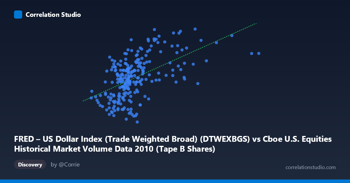
FRED – US Dollar Index (Trade Weighted Broad) (DTWEXBGS) vs Cboe U.S. Equities Historical Market Volume Data 2010 (Tape B Shares)
- Pearson correlation (r)
- 0.5434
- Spearman correlation
- 0.5389
- p-value
- 0
- Sample size (n)
- 245
- 95% confidence interval
- 0.4486 to 0.6261
- Granger causality
- None
- Granger optimal lag
- 1
AI analysis
Scatterplot Analysis: US Dollar Index vs. Cboe Tape B Shares (2010)
Relationship Overview
The scatterplot reveals a moderate positive relationship between the Trade-Weighted US Dollar Index (X-axis) and Cboe Tape B share volume (Y-axis) across 245 trading days in 2010. As the dollar index increases — spanning roughly 37.5 million to 328.6 million in the traded units — Tape B share volume tends to drift upward from approximately 89 to 97.5. The linear regression equation (y = 2.38×10⁻⁸x + 90.36) reflects a very shallow but directionally consistent positive slope, suggesting that periods of a stronger or more actively traded dollar environment coincide with modestly elevated Tape B equity volume. The relationship is visible but clearly not deterministic, with considerable vertical scatter at every level of X.
Correlation Strength and Statistical Interpretation
With r = 0.5434, the correlation is moderate and positive, but the more meaningful metric for practical interpretation is r² = 0.2952 — meaning only about 29.5% of the variance in Tape B share volume is explained by variation in the dollar index. Roughly 70% of the variation in Y remains unexplained by this linear model alone. The 95% confidence interval for r [0.449, 0.626] is reasonably tight given n = 245, and the p-value of effectively 0 confirms this correlation is highly statistically significant and very unlikely to be a chance artifact in the sample. However, statistical significance should not be conflated with practical magnitude — the explained variance is modest at best. Critically, the Granger causality tests reveal no significant temporal predictive direction: X→Y yields F = 0.337, p = 0.562, and Y→X yields F = 3.508, p = 0.062 — both failing conventional significance thresholds. This means neither variable reliably predicts the other one period ahead, which substantially weakens any causal narrative between dollar index movements and Tape B volumes.
Notable Patterns, Clusters, and Outliers
Several features stand out in the sample points. There is a dense cluster of observations in the X range of roughly 60–130 million with Y values between 89 and 95, representing the typical trading day behavior. Above X ≈ 180 million, the data becomes sparser but shows elevated Y values, including notable high-volume outliers such as (218M, 97.55), (228M, 96.51), (147M, 97.50), and (192M, 97.34) — these upper-right points are pulling the regression slope upward and inflating the correlation. Conversely, the point at approximately (37.5M, 91.20) sits at the extreme low end of X without a correspondingly low Y value, suggesting a potential floor effect in Tape B volume. The scatter also reveals heteroscedasticity: variability in Y appears wider at lower X values and somewhat compressed at higher X values, which violates one assumption of standard linear regression and may affect the reliability of the r estimate.
Confounding Factors and Caveats
Several important caveats apply. First, both variables are time series from the same year (2010), so any shared macroeconomic trends — post-financial crisis recovery, Federal Reserve policy, risk-on/risk-off equity cycles — could be driving co-movement in both series simultaneously, creating spurious correlation. Second, the axis labels appear swapped in the dataset metadata (X is labeled as dollar index data but described with equity volume context, and vice versa), which warrants careful verification before drawing any substantive conclusion. Third, N = 3,302 is cited as the population size against n = 245 paired samples, suggesting this analysis covers only a subset of available data; the sampling strategy (every 4th point shown) may introduce gaps that obscure intraday or week-of-year seasonality. Finally, Tape B specifically covers NYSE American and regional exchanges — a narrower slice of market activity — so results may not generalize to total US equity volume.
Actionable Insights and Further Investigation
Despite the modest explanatory power, the correlation is robust enough to warrant deeper investigation. First, researchers should test whether the relationship holds across multiple years, particularly during periods of dollar stress (2008, 2015, 2020), to distinguish a structural relationship from a 2010-specific artifact. Second, controlling for known confounders — VIX (volatility index), Fed funds rate decisions, or S&P 500 return magnitude — in a multivariate regression would clarify whether the dollar index retains independent predictive value for Tape B volume. Third, given the marginal Granger result for Y→X (p = 0.062), it may be worth testing longer lag structures (2–5 periods) to see if Tape B volume has a delayed relationship with dollar index movements. Fourth, the apparent non-linearity and heteroscedasticity suggest that a log transformation of X or a polynomial regression might better capture the true functional form. Finally, verifying the axis/dataset label alignment is an essential data quality step before any further modeling effort.
X dataset: Cboe U.S. Equities Historical Market Volume Data 2010
Y dataset: FRED – US Dollar Index (Trade Weighted Broad)
Part of experiment: Daily - Cboe U.S. Equities Historical Market Volume Data 2010 vs FRED – US Dollar Index (Trade Weighted Broad)