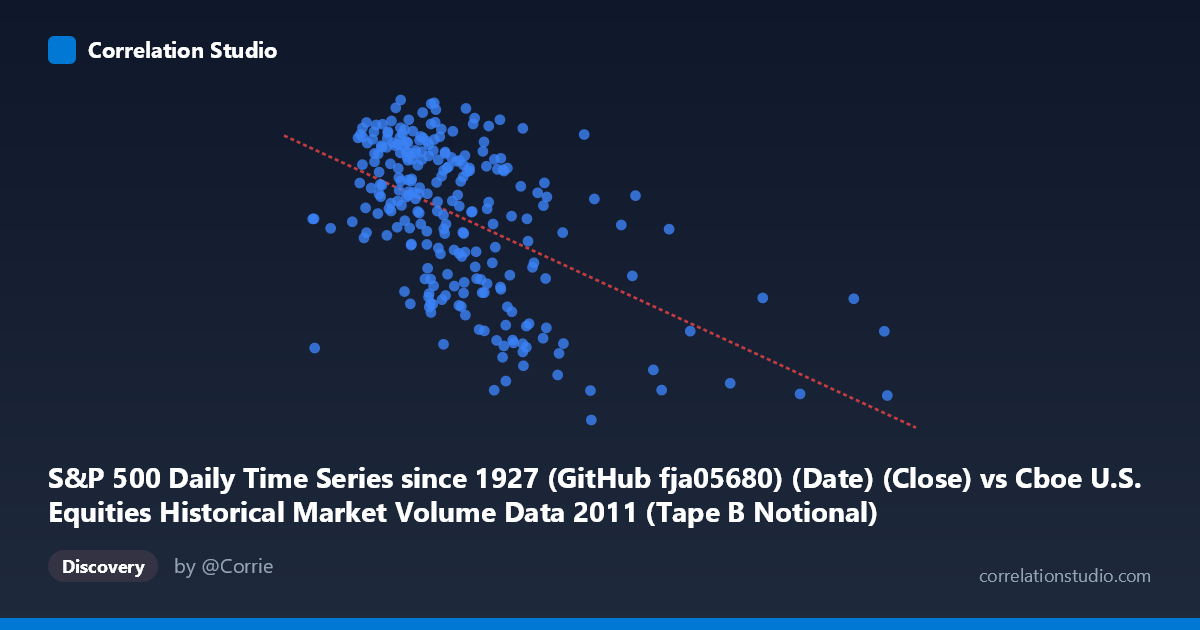
S&P 500 Daily Time Series since 1927 (GitHub fja05680) (Date) (Close) vs Cboe U.S. Equities Historical Market Volume Data 2011 (Tape B Notional)

Pearson correlation (r): -0.5247
Spearman correlation: -0.4926
p-value: 0
Sample size (n): 252
95% confidence interval: -0.6088 to -0.4289
Granger causality: X → Y
Granger optimal lag: 10

AI analysis

Analysis: S&P 500 Close Price vs. Cboe Tape B Notional Volume (2011)

Relationship Overview The scatterplot reveals a negative relationship between S&P 500 closing prices (X-axis, measured in what appear to be date-encoded or scaled values) and Cboe Tape B notional trading volume (Y-axis). As the S&P 500 close price increases, Tape B notional volume tends to decrease, and conversely, lower price levels are associated with higher notional volume. The linear regression equation (y = -1.827×10⁻⁸x + 1361.04) captures this inverse trend, though the scatter around the regression line is substantial, suggesting the relationship is real but far from deterministic. This pattern is consistent with a well-known market microstructure phenomenon: during periods of market stress and declining prices, trading volume and notional activity tend to spike as investors rebalance, hedge, or liquidate positions.

Correlation Strength and Statistical Significance The Pearson correlation of r = -0.5247 indicates a moderate negative correlation, and the R² of 0.2753 means that approximately 27.5% of the variance in Tape B notional volume is explained by the S&P 500 close price level — leaving roughly 72.5% of variance attributable to other factors. The 95% confidence interval of [-0.6088, -0.4289] is entirely negative and does not cross zero, reinforcing that the inverse relationship is statistically robust. The p-value of effectively 0 (with N = 3,780) confirms this is not a chance finding. Critically, the Granger causality analysis points unidirectionally from X→Y (F = 1.88, p = 0.049) at an optimal lag of 10 trading periods, meaning S&P 500 price levels have modest but statistically significant temporal predictive power over subsequent Tape B notional volume roughly two calendar weeks later. The reverse direction (Y→X) shows no such predictive relationship (F = 0.42, p = 0.94), suggesting price changes lead volume responses rather than the other way around in this dataset.

Notable Patterns, Clusters, and Outliers Several features stand out visually. The bulk of observations cluster in the X range of roughly 3.0–6.5 billion (corresponding to mid-2011 S&P price levels), with Y values concentrated between approximately 1,200 and 1,360. There is a notable cluster of high-volume outliers at the lower end of the X range (e.g., points near X ≈ 3.1B with Y ≈ 1,335–1,340), consistent with the market volatility surrounding the August 2011 U.S. debt ceiling crisis and subsequent S&P credit downgrade. On the right tail, a handful of high-X observations (e.g., ~9.5B and ~10.0B) show relatively compressed Y values around 1,170–1,257, suggesting lower notional activity at elevated price levels. Points like (6,102,922,959, 1,131.42) and (6,060,792,168, 1,160.40) appear as potential outliers — unusually low Y values even within their X neighborhood — possibly corresponding to specific low-activity trading sessions (holidays, half-days, or post-crisis calm periods).

Confounding Factors and Interpretive Caveats Several important caveats temper this analysis. First, the X-axis appears to encode dates as Unix timestamps or similar numeric representations, meaning the "correlation" partially reflects a temporal trend — both variables co-evolve over calendar time in 2011, and the correlation may be partly spurious, driven by the shared time dimension rather than a direct causal price-volume mechanism. The Granger test helps address directionality but does not eliminate this concern. Second, Tape B notional volume specifically covers NYSE American (AMEX) and regional exchange listings, not the full market, so it may not perfectly proxy overall market activity. Third, macroeconomic shocks in 2011 (European sovereign debt crisis, U.S. debt ceiling, Federal Reserve communications) likely created regime-specific clusters that inflate the apparent correlation during stress periods. Fourth, the 10-period Granger lag, while statistically significant, has a borderline p-value (0.049), warranting caution about over-interpreting the predictive relationship.

Actionable Insights and Further Investigation Practitioners monitoring equity market microstructure should note that S&P 500 price declines appear to be a leading indicator of elevated Tape B notional volume approximately 10 trading days later, which could inform liquidity provision strategies or risk management timing. However, given that only 27.5% of variance is explained, supplementary variables are essential. Recommended next steps include: (1) decomposing the time series to separate secular trends from cyclical price-volume dynamics; (2) incorporating the VIX or realized volatility as a covariate, since volatility likely mediates much of the price-volume relationship; (3) expanding the analysis across multiple years to test whether the 2011 relationship (heavily influenced by the August crisis) generalizes; and (4) examining whether the relationship holds at intraday resolution or is specific to daily close-to-close measurements. A multivariate regression or VAR model incorporating volatility, market breadth, and macroeconomic regime indicators would likely substantially improve explanatory power beyond the current 27.5%.

X dataset: Cboe U.S. Equities Historical Market Volume Data 2011

Y dataset: S&P 500 Daily Time Series since 1927 (GitHub fja05680) (Date)

Part of experiment: Daily - Cboe U.S. Equities Historical Market Volume Data 2011 vs S&P 500 Daily Time Series since 1927 (GitHub fja05680) (Date)