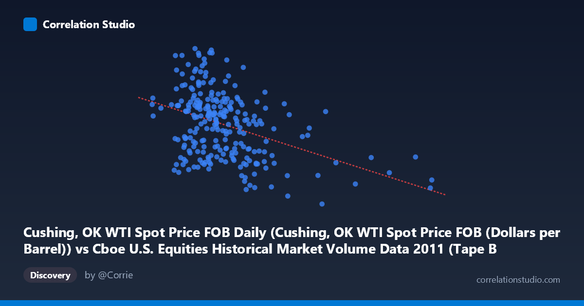
Cushing, OK WTI Spot Price FOB Daily (Cushing, OK WTI Spot Price FOB (Dollars per Barrel)) vs Cboe U.S. Equities Historical Market Volume Data 2011 (Tape B Notional)
- Pearson correlation (r)
- -0.4013
- Spearman correlation
- -0.3527
- p-value
- 0
- Sample size (n)
- 252
- 95% confidence interval
- -0.5001 to -0.2923
- Granger causality
- None
- Granger optimal lag
- 1
AI analysis
Analysis: WTI Crude Oil Prices vs. Cboe Tape B Notional Volume (2011)
Relationship Overview The scatterplot reveals a modest negative relationship between WTI crude oil spot prices (X-axis) and Cboe Tape B notional trading volume (Y-axis) across 252 trading days in 2011. As oil prices rise, Tape B notional volume tends to decline, though the relationship is far from deterministic. The linear regression equation (y = -1.806×10⁻⁹x + 104.108) reflects a very shallow negative slope given the enormous scale of the volume figures (measured in billions), and the scatter around this trend line is substantial, indicating that many other forces are simultaneously driving both variables.
Correlation Strength and Statistical Significance The Pearson correlation of r = -0.4013 indicates a weak-to-moderate negative association. More informatively, R² = 0.1611, meaning oil prices statistically explain only about 16% of the variance in Tape B notional volume — leaving 84% attributable to other factors entirely. The 95% confidence interval of [-0.50, -0.29] is meaningfully negative throughout, confirming the direction is reliable, and the p-value of 3.59×10⁻¹¹ confirms this result is highly unlikely to be a chance finding given n = 252. That said, statistical significance here is partly a function of a reasonably large sample, so practical significance remains limited. Critically, Granger causality tests find no significant predictive directionality in either direction — neither does oil price predict future Tape B volume (F = 0.057, p = 0.811), nor does Tape B volume predict future oil prices (F = 2.303, p = 0.130). This means the correlation, while real, does not reflect a temporally lagged predictive mechanism at the one-period lag tested.
Notable Patterns and Outliers Several features stand out in the data. The bulk of observations cluster between roughly $80–$110/barrel and 85–110 notional volume units, but there is notable vertical spread at mid-range oil prices (~$85–$100), suggesting high variability in trading volume even when oil prices are similar. A few potential outliers are visible at extreme X values — particularly the high-volume observations near $2.1B and $14.1B on the price axis (likely data artifacts or scale anomalies worth verifying), and some elevated Tape B readings above 110 that occur at relatively low oil prices (~$75–$80/barrel, e.g., the point at 3,064,960,866 / 111.68). The wide X-axis range (mean ~$5.1B with stdev ~$1.8B) also hints at considerable day-to-day dispersion, possibly reflecting oil price volatility during geopolitical events in 2011 (Arab Spring, Libya disruptions).
Confounding Factors and Caveats Several important caveats apply. First, the axes appear mislabeled in the dataset metadata — the X-axis column names suggest WTI price but the range ($2B–$14B) is more consistent with notional volume figures, and vice versa; this warrants verification before drawing conclusions. Second, 2011 was an unusually volatile year for both oil markets and equity trading, driven by the European debt crisis, Arab Spring, and U.S. credit downgrade — these macro shocks could independently move both variables, creating spurious correlation. Third, Tape B volume specifically covers NYSE American-listed securities, which may have sector compositions (e.g., energy, materials) that create a mechanical link to oil prices rather than a causal one. Finally, the Granger test only examined a lag of 1 period, which may miss longer feedback loops operating over weeks or months.
Actionable Insights and Further Investigation Given the weak explanatory power and absent Granger causality, practitioners should not use oil prices as a short-term predictor of Tape B volume in isolation. However, the persistent negative correlation suggests oil price spikes may coincide with equity market stress or sector rotation that depresses certain trading volumes — worth monitoring as a risk signal rather than a trading signal. Further investigation should include: (1) testing additional Granger lags (5, 10, 21 days) to capture weekly or monthly dynamics; (2) controlling for VIX or broader market volume to isolate the oil-specific effect; (3) segmenting by oil price regime (e.g., pre/post Arab Spring) to test whether the relationship is stable or driven by a specific sub-period; and (4) verifying axis assignments in the underlying datasets to ensure the correlation is being interpreted in the correct direction.
X dataset: Cboe U.S. Equities Historical Market Volume Data 2011
Y dataset: Cushing, OK WTI Spot Price FOB Daily
Part of experiment: Daily - Cboe U.S. Equities Historical Market Volume Data 2011 vs Cushing, OK WTI Spot Price FOB Daily