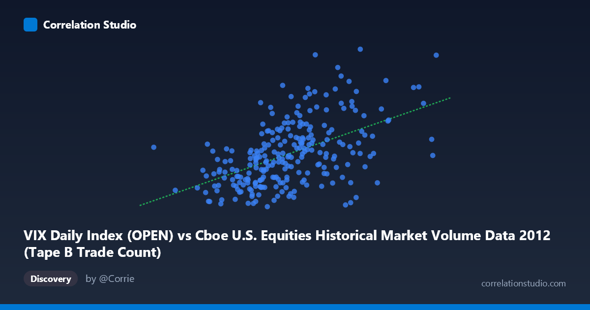
VIX Daily Index (OPEN) vs Cboe U.S. Equities Historical Market Volume Data 2012 (Tape B Trade Count)
- Pearson correlation (r)
- 0.5164
- Spearman correlation
- 0.5263
- p-value
- 0
- Sample size (n)
- 250
- 95% confidence interval
- 0.4192 to 0.6019
- Granger causality
- None
- Granger optimal lag
- 1
AI analysis
Scatterplot Analysis: VIX Daily Index (Open) vs. Tape B Trade Count
Relationship Overview
The scatterplot reveals a moderate positive relationship between the Cboe VIX Daily Index Open values and the Tape B Trade Count for U.S. equities in 2012. As market volume (X) increases, the VIX open level (Y) tends to rise as well, consistent with the well-established financial intuition that heightened trading activity often coincides with elevated market uncertainty or volatility. The linear regression equation (y = 3.36×10⁻⁵x + 12.04) indicates that for every 100,000-unit increase in daily market volume, the VIX is expected to rise by approximately 3.36 points, anchored at a baseline of roughly 12 when volume is negligible — a plausible lower bound given the VIX's historical floor.
Correlation Strength and Statistical Significance
The Pearson correlation of r = 0.5164 reflects a moderate positive association, but the explanatory power deserves careful framing: R² = 0.2667, meaning only about 26.7% of the variance in VIX open levels is explained by Tape B trade count. Roughly three-quarters of VIX variability remains attributable to other factors. The 95% confidence interval for r of [0.419, 0.602] is relatively tight given the sample size of n = 250, and the p-value of effectively zero confirms this correlation is highly statistically significant — not a sampling artifact. However, statistical significance at this scale should not be conflated with practical or causal significance. Critically, Granger causality tests find no significant predictive directionality in either direction (X→Y: F = 3.09, p = 0.080; Y→X: F = 0.15, p = 0.695). The X→Y result narrowly misses conventional significance thresholds (p ≈ 0.08), suggesting a weak temporal signal from volume to VIX, but insufficient to claim reliable predictive causation at a 1-period lag.
Notable Patterns, Clusters, and Outliers
Several features stand out in the data distribution. The bulk of observations cluster in the X range of 130,000–230,000 and Y range of 15–21, forming a moderately dispersed central cloud consistent with typical 2012 trading conditions. However, notable outliers disrupt the trend: the point near (295,122; 17.80) represents extremely high volume but a surprisingly average VIX level, while points such as (222,650; 13.82) and (231,486; 14.42) show high volume paired with unusually low VIX — counterintuitive to the general trend. Conversely, (170,460; 23.44) and (197,126; 22.93) show elevated VIX at only moderate volume levels. These outliers suggest non-linear or regime-dependent dynamics where the volume–volatility relationship may break down under specific market conditions (e.g., low-volatility high-volume days driven by algorithmic or passive flows).
Confounding Factors and Caveats
Several important caveats apply to this analysis. Spurious correlation via shared time-series drivers is a primary concern — both VIX and equity trade counts are influenced by macroeconomic events, Federal Reserve communications, and seasonal market patterns in 2012 (e.g., European debt crisis episodes, U.S. election uncertainty). The relationship may be partly or wholly mediated by these common external shocks rather than reflecting a direct volume–volatility mechanism. Additionally, Tape B specifically covers NYSE American and regional exchanges, representing only a subset of total market activity; using aggregate volume might yield different results. The 2012 time window also limits generalizability — this was a period of recovering but still elevated post-crisis volatility, and correlations may differ substantially in calmer or more turbulent regimes.
Actionable Insights and Further Investigation
Practitioners should treat this correlation as indicative but not predictive given the failed Granger causality tests. For further investigation, several directions are recommended: (1) extend the analysis to multiple years to test whether this r ≈ 0.52 relationship is stable or regime-dependent; (2) decompose by market event type (FOMC days, earnings seasons, macro announcements) to identify whether the outliers cluster around specific catalysts; (3) test non-linear models (e.g., polynomial regression or quantile regression) given the visible heteroscedasticity — the spread in Y appears to widen at moderate X values; and (4) incorporate total consolidated tape volume rather than Tape B alone to assess whether the partial volume measure is attenuating the true relationship. A VAR or structural equation model controlling for macroeconomic co-drivers would also help isolate whether any genuine predictive signal exists between volume and volatility at this lag structure.
X dataset: Cboe U.S. Equities Historical Market Volume Data 2012
Y dataset: VIX Daily Index
Part of experiment: Daily - Cboe U.S. Equities Historical Market Volume Data 2012 vs VIX Daily Index