IMF Primary Commodity Prices – Monthly Time Series (53 Commodities, 10 Indexes) (Palm oil) vs Bitcoin Historical Price USD – All-Time Series (Habrador) (Price)
- Pearson correlation (r)
- -0.4742
- Spearman correlation
- -0.6738
- p-value
- 0.000006
- Sample size (n)
- 83
- 95% confidence interval
- -0.6259 to -0.288
- Granger causality
- None
- Granger optimal lag
- 10
AI analysis
Scatterplot Analysis: Palm Oil Prices vs. Bitcoin Price
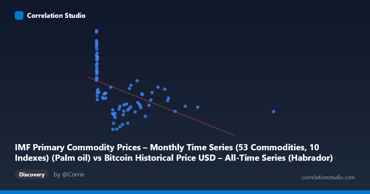
1. Overall Relationship The scatterplot shows a moderate negative relationship between palm oil prices (X-axis) and Bitcoin's USD price (Y-axis). Most data points cluster tightly at low palm oil values (under ~700), with Bitcoin prices spread between roughly 500 and 1250 in this window. A smaller number of high-palm-oil-price points (900–2450) correspond to comparatively lower and more compressed Bitcoin values (around 600–800), pulling the trendline downward and driving the negative slope.
2. Strength, Direction, and Statistical Confidence The Pearson correlation of r = -0.474 indicates a moderate negative linear association, with r² = 0.225 meaning only about 22.5% of the variance in Bitcoin price is explained by palm oil price — leaving roughly 78% attributable to other factors. The 95% CI [-0.626, -0.288] is reasonably tight and entirely negative, and the p-value (5.94E-06) is highly significant, so we can be confident a real (non-zero) negative association exists in this sample — but the practical predictive power is limited given the modest r². Critically, the Granger causality tests show no significant predictive direction in either direction (X→Y p=0.445; Y→X p=0.323), meaning historical values of one series do not meaningfully forecast future values of the other at the tested lag. This suggests the correlation is likely coincidental, driven by a shared external trend (e.g., both series evolving over the 2010–2017 period) rather than a genuine causal or lead-lag relationship.
3. Patterns, Clusters, and Outliers The data is heavily clustered in the low-X region (palm oil < 700), with a dense concentration of points near X < 50 showing a wide vertical spread in Bitcoin price (500 to 1250) — this vertical scatter at low X suggests that when palm oil is low, Bitcoin price is highly variable and not well constrained by palm oil alone. A sparser set of high-leverage points exist at X 900 (up to 2452), which have outsized influence on the regression slope despite being few in number — removing these could substantially change the fitted line. The note that Spearman's ρ exceeds Pearson's r hints at a non-linear (possibly logarithmic or power-law) relationship, consistent with the compressed, saturating pattern of Y at high X values — a log-transform of X may produce a better and more stable fit.
4. Confounding Factors and Caveats This is a classic case of two unrelated time series that both trend over time, risking spurious correlation: Bitcoin's price underwent dramatic secular growth (and volatility) from 2010–2017 independent of commodity markets, while palm oil prices follow their own agricultural/economic cycles. Neither has an obvious economic mechanism tying them together. The small sample size (n=83 paired points vs. N=449 available) and uneven time-density (heavy clustering at low X) further limit generalizability. Autocorrelation within each time series (common in financial/commodity data) can inflate apparent correlation significance beyond what independent observations would justify.
5. Recommendations for Further Investigation Given the lack of Granger causality, this pairing should not be used for forecasting purposes. Instead: (1) test a log or polynomial transform of X per the Spearman/Pearson discrepancy to check if a non-linear model improves r² meaningfully; (2) run the analysis on returns/differences rather than levels to control for shared trending and autocorrelation, which often eliminates spurious relationships; (3) explicitly test for a common confounder (e.g., overall USD strength, global risk sentiment, or time itself) using partial correlation; and (4) increase the sample density in the underrepresented high-X region to verify whether the negative slope holds or is an artifact of a few leverage points.
X dataset: Bitcoin Historical Price USD – All-Time Series (Habrador)
Y dataset: IMF Primary Commodity Prices – Monthly Time Series (53 Commodities, 10 Indexes)
Part of experiment: Bitcoin - Bitcoin Historical Price USD – All-Time Series (Habrador) vs IMF Primary Commodity Prices – Monthly Time Series (53 Commodities, 10 Indexes)