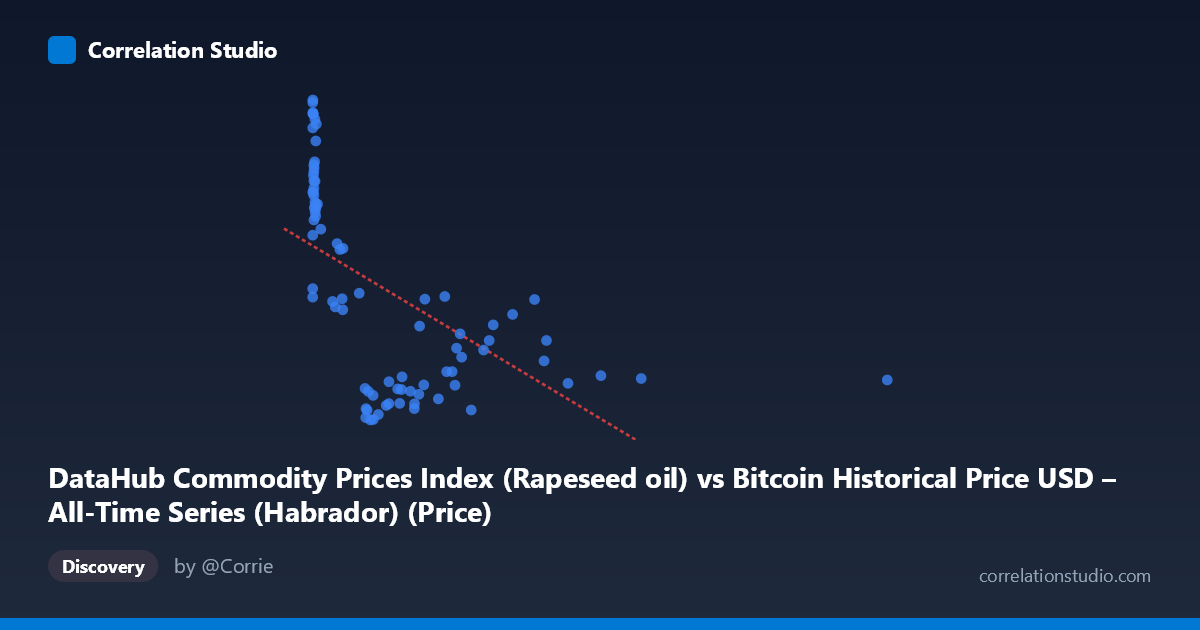
DataHub Commodity Prices Index (Rapeseed oil) vs Bitcoin Historical Price USD – All-Time Series (Habrador) (Price)
- Pearson correlation (r)
- -0.5688
- Spearman correlation
- -0.702
- p-value
- 0
- Sample size (n)
- 83
- 95% confidence interval
- -0.6988 to -0.4025
- Granger causality
- None
- Granger optimal lag
- 10
AI analysis
Analysis: Rapeseed Oil Price Index vs. Bitcoin Price (USD)
1. Overall Relationship
The scatterplot shows a moderate negative relationship between the rapeseed oil commodity index (X) and Bitcoin's historical price (Y). Rather than a clean linear decline, the data forms a distinctive L-shaped or hyperbolic pattern: a dense vertical cluster of points at very low X values (near 0–50) spans a huge range of Y (roughly 950–1450), while as X increases beyond ~200–2450, Y compresses into a much narrower, lower band (~750–1050). This shape—high variance at low X, low variance at high X—is the classic signature of an inverse or logarithmic relationship rather than a straight-line one.
2. Strength, Direction, and Statistical Confidence
The Pearson correlation (r = -0.569, R² = 0.324) indicates a moderate negative linear association, explaining about 32% of the variance in Y. The 95% CI [-0.699, -0.403] excludes zero and is reasonably tight, and the p-value (2.0×10⁻⁸) is highly significant, so we can be confident a real negative association exists in this sample — this is not noise. However, R² of 0.32 also means 68% of Bitcoin price variance is left unexplained by rapeseed oil prices alone, so the relationship, while statistically robust, has limited practical predictive power on its own. Critically, the Granger causality tests (both directions non-significant: X→Y p=0.838, Y→X p=0.173) show no evidence that either series temporally predicts the other. This strongly suggests the correlation is not causal in either direction — it's more likely a spurious or coincidental co-movement, possibly driven by both series trending over the same calendar period (2010–2017) for unrelated reasons.
3. Notable Patterns and Outliers
The most striking feature is the asymmetric clustering: dozens of points sit at X < 20 with Y ranging widely from ~950 to ~1450 (early low-volume commodity readings paired with a wide spread of Bitcoin prices across different months/years). In contrast, mid-to-high X values (300–2452) correspond almost exclusively to Y in the 750–1050 range, with much less scatter. The single point at X = 2452.18 (Y = 830) is a clear high-leverage outlier, sitting far from the rest of the X distribution and likely exerting outsized influence on the linear fit. The note that Spearman ρ exceeds Pearson r reinforces that a monotonic but curved (logarithmic or power-law) relationship fits better than a straight line — consistent with the visual L-shape.
4. Confounding Factors and Caveats
Both variables are time series spanning 2010–2017, a period during which Bitcoin underwent enormous, non-stationary price swings (from cents to thousands of dollars) largely driven by adoption cycles, exchange dynamics, and speculative bubbles — factors entirely unrelated to rapeseed oil markets. Any apparent correlation between an unrelated commodity index and Bitcoin over this window is a common trap of time-series analysis: two independent trending series can show statistically significant correlation purely by chance (spurious regression), especially with autocorrelated, non-stationary data. The lack of Granger causality strongly supports this interpretation. Sample size (n=83 paired points) is also much smaller than the full population (N=449), and the extreme value at X≈2452 could be disproportionately driving the linear r estimate.
5. Actionable Insights
Given the absence of Granger causality and the biologically/economically implausible link between rapeseed oil and Bitcoin, this correlation should be treated as likely spurious rather than a tradable or causal signal. Recommended next steps: (1) test both series for stationarity (ADF test) and consider differencing or detrending before any causal inference, since raw trending series inflate correlation artificially; (2) refit using a log or power-law model given the L-shaped pattern and Spearman-Pearson discrepancy; (3) examine whether a hidden common factor (e.g., global risk sentiment, USD strength, or simple calendar-time trend) better explains both series' movements; and (4) exclude or separately analyze the extreme outlier at X=2452 to check its influence on the reported r and slope.
X dataset: Bitcoin Historical Price USD – All-Time Series (Habrador)
Y dataset: DataHub Commodity Prices Index
Part of experiment: Bitcoin - Bitcoin Historical Price USD – All-Time Series (Habrador) vs DataHub Commodity Prices Index