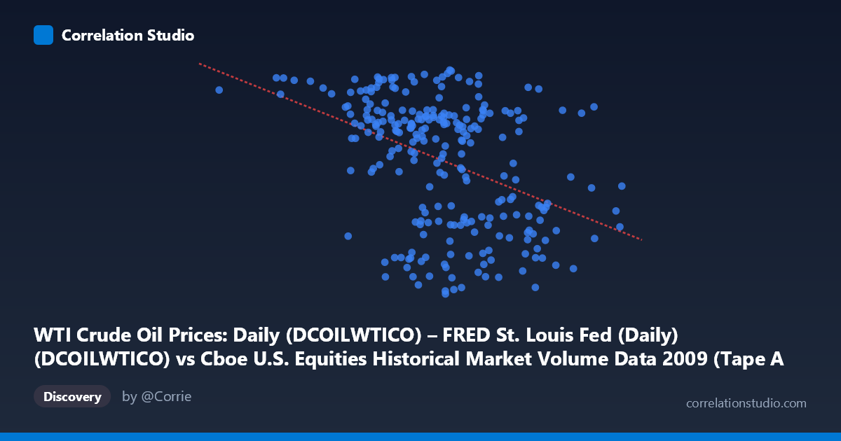
WTI Crude Oil Prices: Daily (DCOILWTICO) – FRED St. Louis Fed (Daily) (DCOILWTICO) vs Cboe U.S. Equities Historical Market Volume Data 2009 (Tape A Shares)
- Pearson correlation (r)
- -0.407
- Spearman correlation
- -0.3948
- p-value
- 0
- Sample size (n)
- 250
- 95% confidence interval
- -0.5055 to -0.298
- Granger causality
- None
- Granger optimal lag
- 1
AI analysis
Analysis: WTI Crude Oil Prices vs. Cboe U.S. Equities Market Volume (2009)
Relationship Overview The scatterplot reveals a moderate negative relationship between WTI crude oil prices and Cboe U.S. equities market volume (Tape A Shares) across 252 trading days in 2009. As crude oil prices increase, equity trading volume tends to decline, and vice versa. The linear regression equation (y = -5.66×10⁻⁸x + 86.82) confirms this downward slope, though the scatter around the regression line is substantial, indicating considerable unexplained variability. Visually, the data points form a diffuse cloud with a gentle negative tilt rather than a tight, well-defined linear band — a pattern consistent with a real but modest association.
Correlation Strength and Statistical Significance The Pearson correlation of r = -0.414 indicates a moderate negative association, but the coefficient of determination (r² = 0.171) is the more sobering figure: only 17.1% of the variance in equity trading volume is explained by WTI crude oil prices. The remaining ~83% is attributable to other factors entirely. The 95% confidence interval of [-0.511, -0.306] is meaningfully negative throughout — it does not cross zero — and the p-value of 7.49×10⁻¹² confirms this result is highly statistically significant at the n = 252 sample level, making a chance finding extremely unlikely. However, statistical significance here is partly a function of a reasonably large sample, and practical significance remains modest. Critically, Granger causality tests show no significant predictive directionality in either direction (X→Y: F = 0.47, p = 0.49; Y→X: F = 0.07, p = 0.79), meaning that past crude oil prices do not help predict future equity volume, and past volume does not help predict future oil prices at the optimal 1-period lag. This absence of Granger causality tempers any interpretation of a causal or even temporally predictive mechanism between these variables.
Patterns, Clusters, and Outliers Several structural features are visible in the scatterplot. There appear to be two loose clusters in the data: one grouping at lower oil prices (roughly $35–$55/barrel) where equity volumes span a wide range, and another at higher prices ($55–$75/barrel) where volumes tend to cluster at lower levels — consistent with the negative trend. A handful of notable outliers stand out, particularly points with very high equity volumes (above ~78–81 billion shares) occurring across a range of oil price levels, including both low and moderate prices (e.g., ~$105M→76.83, ~$201M→79.35, ~$362M→78.91, ~$411M→80.11). There is also a point at the extreme right of the X-axis (~$704M oil price equivalent) with moderate volume (~56.67), which anchors the regression but may exert disproportionate leverage. The spread of Y values at any given X level is wide (~34 to ~81), reinforcing that the relationship is noisy and non-deterministic.
Confounding Factors and Caveats Several important caveats apply. First, 2009 was a highly anomalous year — the global financial crisis recovery, extraordinary market volatility, quantitative easing, and oil price rebounds from their 2008 crash lows all overlapped, making this period structurally unusual and potentially non-generalizable. Second, both variables were likely driven by common macro factors (risk sentiment, economic recovery expectations, institutional flows) rather than directly influencing each other — classic spurious correlation via omitted confounders such as VIX (fear index), S&P 500 returns, or Federal Reserve policy signals. Third, the axis labels appear to be swapped in the dataset metadata (the X-axis description references FRED WTI oil prices but is labeled as Cboe volume data, and vice versa), which warrants data verification before drawing firm conclusions. Finally, daily data introduces autocorrelation within each series that can inflate apparent statistical significance if not properly accounted for.
Actionable Insights and Further Investigation Despite the modest r², the consistent negative correlation and high statistical significance suggest this relationship warrants structured follow-up. Analysts should consider: (1) incorporating VIX or S&P 500 returns as control variables in a multivariate regression to test whether the oil-volume relationship persists after accounting for broader market risk sentiment; (2) conducting rolling-window correlation analysis to determine whether this relationship was stronger during specific 2009 sub-periods (e.g., Q1 crisis trough vs. Q3–Q4 recovery); (3) exploring non-linear models (e.g., polynomial or regime-switching), given the visual suggestion of heteroscedasticity and clustering; (4) extending the analysis across multiple years to test whether the 2009 result reflects a stable structural relationship or a crisis-specific artifact; and (5) verifying and correcting the apparent dataset column mapping discrepancy to ensure the axes represent what is analytically intended.
X dataset: Cboe U.S. Equities Historical Market Volume Data 2009
Y dataset: WTI Crude Oil Prices: Daily (DCOILWTICO) – FRED St. Louis Fed (Daily)
Part of experiment: Daily - Cboe U.S. Equities Historical Market Volume Data 2009 vs WTI Crude Oil Prices: Daily (DCOILWTICO) – FRED St. Louis Fed (Daily)