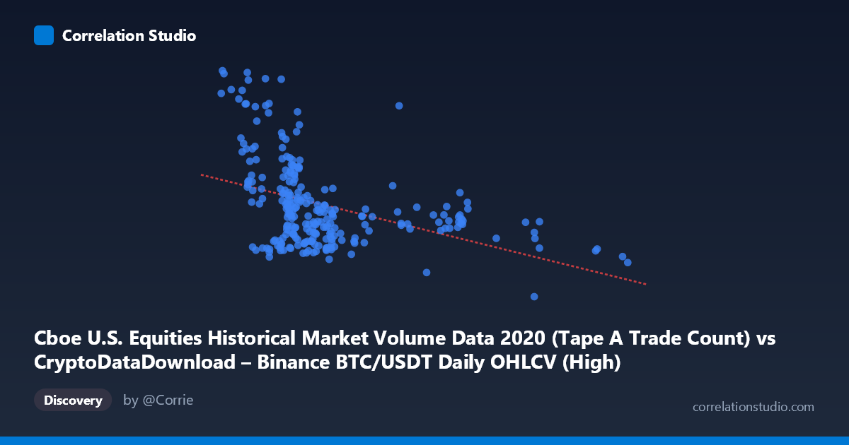
Cboe U.S. Equities Historical Market Volume Data 2020 (Tape A Trade Count) vs CryptoDataDownload – Binance BTC/USDT Daily OHLCV (High)
- Pearson correlation (r)
- -0.4186
- Spearman correlation
- -0.4642
- p-value
- 0
- Sample size (n)
- 253
- 95% confidence interval
- -0.5153 to -0.3113
- Granger causality
- None
- Granger optimal lag
- 10
AI analysis
Analysis: Trade Count vs. BTC/USDT Daily High
1. What the Visualization Reveals
The scatterplot displays a weak-to-moderate negative relationship between Cboe U.S. equities trade counts (X) and the daily high price of BTC/USDT (Y). Most observations cluster tightly in the X range of 7,000–12,000, with Y values scattered widely between roughly 1.2M and 2.9M. A smaller, sparser tail of points extends out to X values of 18,000–29,300, and these high-X points tend to correspond to lower Y values, which is largely driving the negative slope. The bulk of the data cloud, however, shows substantial vertical scatter at any given X, indicating that X alone is a weak predictor of Y within the dense cluster.
2. Strength, Direction, and Statistical Meaning
The correlation coefficient (r = -0.4186) indicates a moderate negative linear relationship, but r² = 0.1752 means only about 17.5% of the variance in Y is explained by X — the remaining 82.5% is attributable to other factors or noise. The 95% CI [-0.5153, -0.3113] is reasonably tight and excludes zero, and the p-value (3.745E-12) confirms this correlation is highly statistically significant and not a product of chance, given n=253. However, statistical significance should not be conflated with practical strength: this is a modest relationship, not one from which precise predictions can be made. Critically, the Granger causality tests show no significant predictive direction in either direction (X→Y: p=0.8485; Y→X: p=0.4265) even at an optimal lag of 10 periods. This strongly suggests the correlation is contemporaneous/coincidental rather than causal in a temporal-lead sense — neither series helps forecast the other's future values.
3. Notable Patterns and Outliers
The data shows a clear bimodal density structure: a dense cluster at low X (7,000–13,000) with high Y variance, and a sparse, more linear-looking tail at high X (18,000–29,300) with consistently lower Y values (~1.2M–1.9M). This tail may disproportionately influence the correlation coefficient and regression slope — a classic leverage-point scenario. Within the main cluster, there are notable high-Y outliers (e.g., points near 2.8M–3.2M at X≈6,600–9,900) that appear disconnected from any strong X pattern, suggesting these price spikes were driven by factors unrelated to equity trade volume. The relationship also looks non-linear/heteroscedastic: variance in Y shrinks as X increases, hinting the true relationship may be better modeled as a threshold or funnel-shaped pattern rather than strictly linear.
4. Confounding Factors and Caveats
Both series are time-stamped daily data from 2020 — a year dominated by COVID-19 market shocks, unprecedented monetary stimulus, and a historic bull run in BTC. Both equities trading activity and crypto prices were likely responding to shared macro drivers (liquidity injections, retail trading surges, risk sentiment) rather than one causing the other. This is a textbook case of potential spurious correlation via a common confounder (e.g., overall market volatility, VIX, retail participation trends, or calendar effects like the March 2020 crash). Additionally, comparing a trade-count metric (equities) to a price-level metric (crypto) mixes fundamentally different economic quantities — units and scale mismatches make causal interpretation tenuous.
5. Actionable Insights
Given the lack of Granger causality, this pairing should not be used for predictive/trading models assuming one series leads the other. Further investigation should: (a) test the relationship using returns/changes rather than levels to reduce trend-driven spurious correlation, (b) introduce control variables like VIX, BTC trading volume, or macro liquidity indices to check if the correlation survives after conditioning, (c) examine whether removing the high-X tail (18k–29k) changes the correlation materially, since it may be an artifact of a few clustered days (possibly around high-volatility events like March 2020), and (d) explore non-linear or lagged-window models given the funnel-shaped variance pattern observed.
X dataset: CryptoDataDownload – Binance BTC/USDT Daily OHLCV
Y dataset: Cboe U.S. Equities Historical Market Volume Data 2020
Part of experiment: Bitcoin - CryptoDataDownload – Binance BTC/USDT Daily OHLCV vs Cboe U.S. Equities Historical Market Volume Data 2020