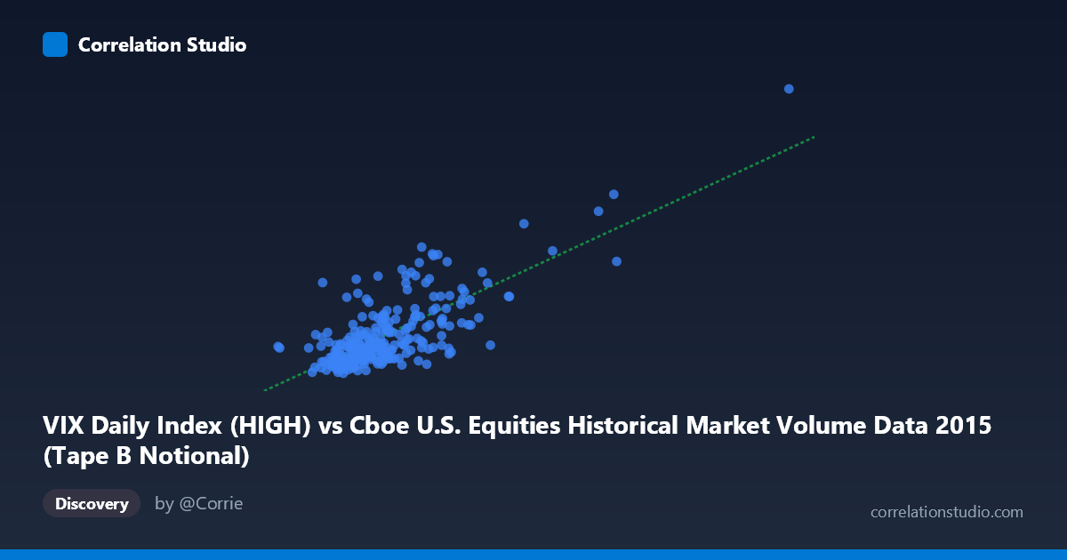
VIX Daily Index (HIGH) vs Cboe U.S. Equities Historical Market Volume Data 2015 (Tape B Notional)
- Pearson correlation (r)
- 0.7469
- Spearman correlation
- 0.632
- p-value
- 0
- Sample size (n)
- 252
- 95% confidence interval
- 0.6867 to 0.7969
- Granger causality
- None
- Granger optimal lag
- 1
AI analysis
Analysis: VIX Daily Index (HIGH) vs. Tape B Notional Volume (2015)
Relationship Overview The scatterplot reveals a moderately strong positive relationship between the VIX Daily Index High values and Tape B Notional trading volume across U.S. equity exchanges in 2015. As the VIX — a widely-followed measure of expected market volatility — rises, Tape B Notional volume tends to increase correspondingly. This is intuitively coherent: elevated fear or uncertainty in markets typically drives heightened trading activity, as investors reposition portfolios, hedge exposures, or react to news-driven price swings. The linear regression equation (y = 2.16e-9·x + 5.999) confirms a positive slope, with the intercept suggesting a baseline VIX level of roughly 6 even at negligible volume — though this is an extrapolation well outside the data range and should not be interpreted literally.
Correlation Strength and Statistical Significance The Pearson correlation of r = 0.7469 indicates a moderately strong positive association, and the R² = 0.5579 means that approximately 55.8% of the variance in VIX highs is explained by Tape B Notional volume (or vice versa). While this is a meaningful explanatory share, it also highlights that roughly 44% of VIX variation is attributable to other factors not captured in this single predictor. The 95% confidence interval of [0.6867, 0.7969] is relatively narrow given the sample size of n = 252, and the p-value of effectively zero confirms this correlation is highly unlikely to be a statistical artifact. However, the Granger causality tests reveal no significant temporal predictive direction in either direction (X→Y: F = 0.082, p = 0.775; Y→X: F = 0.198, p = 0.657), meaning that neither variable reliably predicts the other's future values at a one-period lag. This is a critical distinction: the variables move together, but neither leads the other in a temporally exploitable way.
Notable Patterns, Clusters, and Outliers The sample points reveal a distinct clustering of observations in the lower-left region — VIX values in the 12–20 range paired with notional volumes between roughly 3.2B and 6.2B — reflecting the relatively calm market conditions that dominated much of early-to-mid 2015. However, a clearly visible upper-right cluster of outliers emerges, with points such as (12.58B, 28.38), (12.49B, 38.06), and (9.24B, 23.33) representing periods of significantly elevated volatility and volume simultaneously. The point at approximately (12.49B, 38.06) is particularly notable — likely corresponding to the August 2015 market correction — and may be exerting disproportionate leverage on the regression slope. The relationship also appears to fan outward at higher X values, hinting at possible heteroscedasticity, where variance in VIX increases as notional volume rises.
Confounding Factors and Caveats Several important caveats apply. First, the axis assignment warrants scrutiny: VIX data is on the X-axis while Tape B Notional (an equity market volume metric) is on the Y-axis, yet conceptually, one might expect VIX — as a forward-looking fear gauge — to be the dependent variable. The labeling in the dataset metadata also appears potentially swapped (Tape B Notional is drawn from the "VIX Daily Index" dataset and vice versa), which could reflect a data-joining artifact. Second, 2015 was a structurally unusual year, bookended by the August flash crash and China-driven volatility spikes, meaning this correlation may not generalize across other calendar years. Third, common macro drivers — such as Federal Reserve policy uncertainty, geopolitical events, or sector-specific shocks — likely inflate both variables simultaneously, creating the appearance of a direct relationship when both may be responding to a shared latent factor. Finally, the absence of Granger causality at lag-1 suggests the relationship is contemporaneous rather than predictive, limiting its use for trading signals.
Actionable Insights and Further Investigation Practitioners should explore lagged cross-correlations at multiple lag lengths beyond lag-1 to determine whether any delayed predictive signal exists at weekly or multi-day horizons. Decomposing the data by market regime (e.g., low-vol vs. high-vol periods using VIX thresholds of 15 and 25) would reveal whether the correlation holds uniformly or is driven primarily by the outlier cluster around the August correction. Additionally, residual analysis of the linear regression should be conducted to formally test for heteroscedasticity and non-linearity — a log transformation of the X variable or a piecewise regression may substantially improve model fit. Finally, incorporating additional Tape categories (A and C) alongside macro controls (e.g., S&P 500 returns, Fed meeting dates) in a multivariate framework would help isolate how much of the explained variance is genuinely attributable to VIX dynamics versus confounding market-wide forces.
X dataset: Cboe U.S. Equities Historical Market Volume Data 2015
Y dataset: VIX Daily Index
Part of experiment: Daily - Cboe U.S. Equities Historical Market Volume Data 2015 vs VIX Daily Index