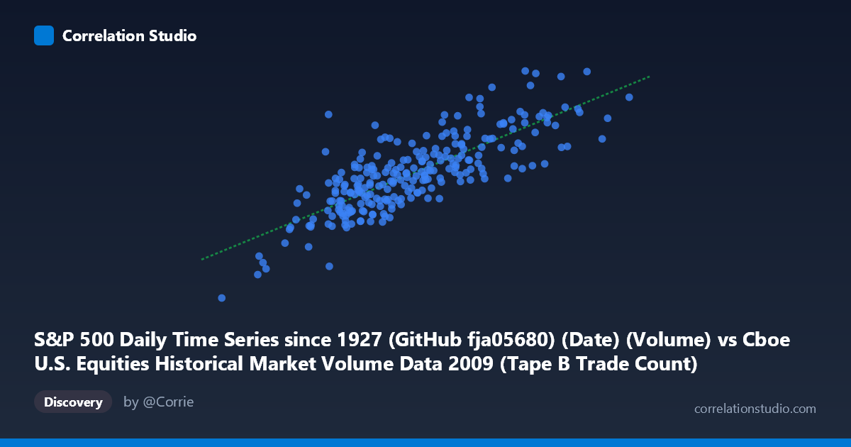
S&P 500 Daily Time Series since 1927 (GitHub fja05680) (Date) (Volume) vs Cboe U.S. Equities Historical Market Volume Data 2009 (Tape B Trade Count)
- Pearson correlation (r)
- 0.7965
- Spearman correlation
- 0.7808
- p-value
- 0
- Sample size (n)
- 252
- 95% confidence interval
- 0.7464 to 0.8376
- Granger causality
- None
- Granger optimal lag
- 10
AI analysis
Scatterplot Analysis: S&P 500 Daily Volume vs. Cboe Tape B Trade Count (2009)
Relationship Overview The scatterplot reveals a moderately strong positive linear relationship between S&P 500 daily trading volume and Cboe U.S. Equities Tape B trade count across the 2009 trading year. As daily volume increases, Tape B trade counts rise correspondingly, which is intuitively consistent — higher overall market activity tends to lift transaction counts across all reporting tapes. The linear regression equation (y = 8,404.43x + 2.196B) suggests that for every unit increase in S&P 500 volume, Tape B trade count increases by approximately 8,404 trades, with a substantial baseline intercept reflecting persistent baseline trading activity even at lower volume levels.
Correlation Strength and Statistical Significance The Pearson correlation of r = 0.7965 indicates a strong positive association, and the r² of 0.6344 means that roughly 63.4% of the variance in Tape B trade count is explained by S&P 500 volume alone — a meaningful but incomplete explanation, leaving ~37% attributable to other factors. The 95% confidence interval of [0.7464, 0.8376] is relatively tight, reflecting high precision given the sample of n = 252 trading days drawn from a population of N = 3,232. The p-value of essentially zero confirms this relationship is highly statistically significant and almost certainly not due to chance. However, the Granger causality analysis complicates the picture: neither direction (X→Y nor Y→X) achieves significance at the optimal 10-period lag (F = 0.50, p = 0.89 for X→Y; F = 1.31, p = 0.23 for Y→X). This means that despite a strong contemporaneous correlation, neither variable reliably predicts the other in a temporal sense — the relationship is concurrent rather than directional or causal.
Notable Patterns, Clusters, and Outliers The data displays a reasonably well-behaved linear cloud with moderate scatter, but several features stand out. There is a visible lower-left cluster anchored by the clear outlier at approximately (81,703; 1.27B) and another low-value point near (156,192; 2.28B), which appear to represent unusually low-volume days — possibly holiday-adjacent sessions or early 2009 market disruption periods. At the upper end, points such as (591,944; 9.12B) and (652,130; 8.93B) represent high-volume, high-trade-count sessions, consistent with the heightened volatility of 2009's recovery period. Notably, the spread around the regression line widens at higher volume levels, suggesting mild heteroscedasticity — variance in Tape B trade counts increases as volume rises, which is common in financial time series where extreme days are more unpredictable.
Confounding Factors and Caveats Several confounding factors warrant caution. First, 2009 was an exceptional year — spanning the tail of the global financial crisis and a historic market recovery from March lows — meaning structural volatility shifts may create spurious or amplified correlations not representative of normal market conditions. Second, both variables are likely driven by a common latent factor: overall market sentiment or macroeconomic news flow. When a major event (e.g., Fed announcement, earnings season) hits, both volume and trade counts rise together, making it difficult to attribute the correlation to any direct mechanism between these two specific series. Third, the Tape B designation covers specific exchanges (e.g., regional exchanges, NYSE American), so its trade count reflects a subset of market activity, and compositional shifts in where trading occurs during 2009 (e.g., fragmentation effects, rise of dark pools) could introduce noise or structural breaks in the relationship.
Actionable Insights and Further Investigation Given that ~37% of Tape B trade count variance remains unexplained, incorporating additional predictors — such as VIX levels, bid-ask spreads, or intraday volatility measures — into a multivariate model would likely improve explanatory power and offer more practical forecasting utility. The absence of Granger causality suggests these variables should be modeled as jointly dependent on external drivers rather than as a predictive pipeline, making vector autoregression (VAR) with exogenous volatility inputs a reasonable next step. Researchers should also test whether the relationship holds outside of 2009 or across different market regimes, given the year's extraordinary character. Finally, investigating the apparent heteroscedasticity formally (e.g., Breusch-Pagan test) and considering a log-log transformation of both variables could stabilize variance and potentially reveal a more robust underlying power-law relationship between volume and trade count.
X dataset: Cboe U.S. Equities Historical Market Volume Data 2009
Y dataset: S&P 500 Daily Time Series since 1927 (GitHub fja05680) (Date)
Part of experiment: Daily - Cboe U.S. Equities Historical Market Volume Data 2009 vs S&P 500 Daily Time Series since 1927 (GitHub fja05680) (Date)