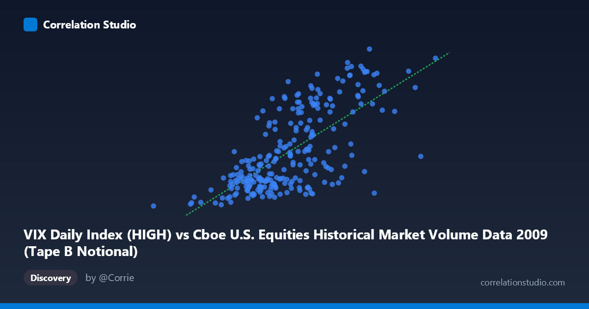
VIX Daily Index (HIGH) vs Cboe U.S. Equities Historical Market Volume Data 2009 (Tape B Notional)
- Pearson correlation (r)
- 0.6952
- Spearman correlation
- 0.6745
- p-value
- 0
- Sample size (n)
- 252
- 95% confidence interval
- 0.6254 to 0.754
- Granger causality
- None
- Granger optimal lag
- 1
AI analysis
Analysis: VIX Daily Index (HIGH) vs. Tape B Notional Trading Volume (2009)
Relationship Overview The scatterplot reveals a moderate positive relationship between the VIX Daily Index High values and Tape B Notional trading volume across U.S. equities exchanges in 2009. As VIX High readings increase, Tape B Notional volume tends to rise correspondingly, which aligns intuitively with market microstructure theory: elevated volatility typically drives greater trading activity as investors rebalance, hedge, or react to uncertainty. The linear regression equation (y = 5.11×10⁻⁹x + 5.84) reflects this positive slope, though the relationship is clearly not perfectly linear — substantial scatter is visible throughout the plot, particularly at mid-range VIX values.
Correlation Strength and Statistical Significance The Pearson correlation of r = 0.6952 indicates a moderately strong positive association. However, the coefficient of determination r² = 0.4833 is the more sobering metric: only 48.3% of the variance in Tape B Notional volume is explained by the VIX High level, meaning over half the variation in trading volume is attributable to other factors entirely. The 95% confidence interval of [0.6254, 0.7540] is reasonably tight and excludes zero, and the p-value of effectively 0 (given n = 252, N = 3,232) confirms this correlation is highly unlikely to be a sampling artifact. That said, Granger causality tests reveal no significant predictive directionality in either direction — neither X→Y (F = 0.013, p = 0.911) nor Y→X (F = 0.195, p = 0.659) — meaning that past VIX values do not predict future Tape B volume, nor vice versa, at a one-period lag. This is a critical caveat: the correlation is contemporaneous, not predictive.
Notable Patterns and Outliers Several structural features stand out in the data. There appears to be a dense cluster of points at lower VIX levels (roughly 20–30) and moderate volume values, consistent with the relative market calm of mid-to-late 2009 following the crisis peak. A secondary, more dispersed cluster emerges at higher VIX readings (40–57), corresponding to elevated volumes — likely reflecting the residual volatility and heavy trading activity from early 2009's bear market bottom and recovery. A handful of high-leverage outliers are visible at the upper-right quadrant (e.g., VIX ≈ 57, Tape B Notional ≈ 9.5B), which could exert disproportionate influence on the regression slope. Notably, the point at the extreme low end (VIX ≈ 19.67, volume ≈ 1.32B) also stands somewhat apart, potentially representing an unusually quiet late-year trading session.
Confounding Factors and Caveats Several confounds deserve careful consideration. 2009 was an exceptional market year — spanning the tail end of the global financial crisis and a dramatic recovery — meaning the VIX range captured here (19.67 to 57.36) reflects a historically extreme volatility regime rather than typical conditions; results may not generalize to other years. The axis labels appear to be swapped between the dataset descriptions (VIX High is on the X-axis despite being sourced from the "Cboe Market Volume" dataset label, and vice versa), suggesting a possible metadata inconsistency worth verifying before drawing conclusions. Additionally, Tape B specifically covers NYSE American-listed securities, so volume dynamics here may differ from broader market behavior. Calendar effects, macroeconomic announcements, and options expiration cycles are all potential confounders driving both VIX and volume simultaneously — a classic common-cause (spurious) correlation scenario where a third variable (e.g., market stress events) drives both metrics.
Actionable Insights and Further Investigation Given the moderate r² and absence of Granger causality, practitioners should avoid using VIX levels as a leading indicator for Tape B volume prediction at a one-day lag. However, the contemporaneous relationship is strong enough to warrant intraday or same-day modeling where VIX can serve as a useful control variable in volume forecasting models. It would be valuable to extend the Granger causality test to longer lags (2–5 periods) to rule out delayed predictive effects. Decomposing the data by market regime (crisis period: Jan–March vs. recovery: April–December) would likely reveal meaningfully different correlation structures. Finally, incorporating additional predictors — such as S&P 500 returns, options expiration dates, and Fed announcement days — into a multivariate regression could substantially improve on the 48.3% variance explained and provide more operationally useful volume forecasting models.
X dataset: Cboe U.S. Equities Historical Market Volume Data 2009
Y dataset: VIX Daily Index
Part of experiment: Daily - Cboe U.S. Equities Historical Market Volume Data 2009 vs VIX Daily Index