IMF Primary Commodity Prices – Monthly Time Series (53 Commodities, 10 Indexes) (Zinc) vs Bitcoin Historical Price USD – All-Time Series (Habrador) (Price)
- Pearson correlation (r)
- 0.4717
- Spearman correlation
- 0.1861
- p-value
- 0.000007
- Sample size (n)
- 83
- 95% confidence interval
- 0.2851 to 0.624
- Granger causality
- None
- Granger optimal lag
- 10
AI analysis
Analysis: Zinc Prices vs. Bitcoin Historical Price
1. What the Visualization Reveals
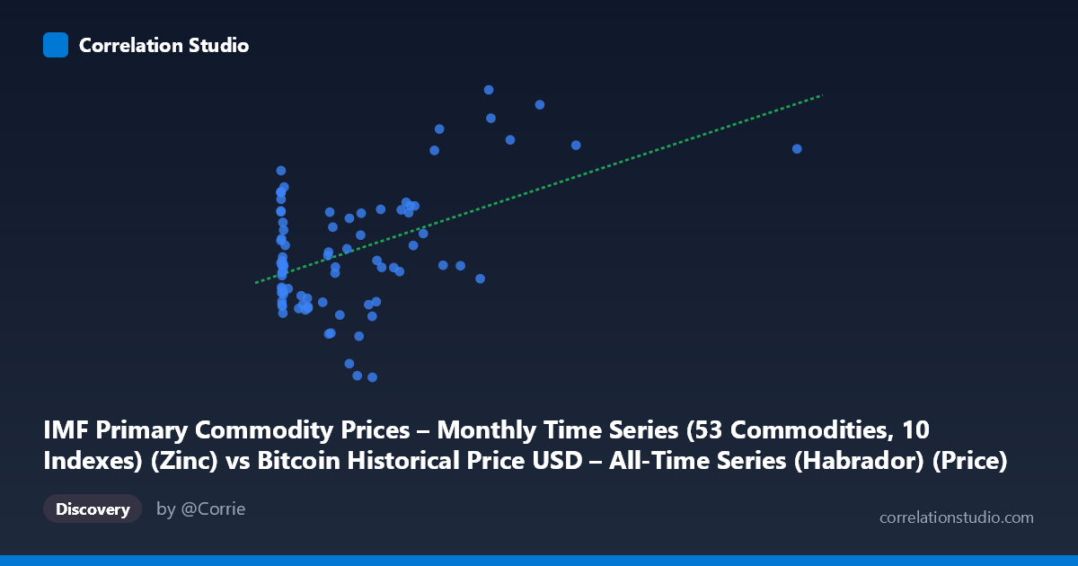
The scatterplot shows a moderate positive relationship between zinc commodity prices (X-axis) and Bitcoin price (Y-axis) over the 2010–2017 period. Most data points cluster tightly at low X-values (roughly 0–700 on the zinc index), with Bitcoin prices ranging widely from ~1,520 to ~2,850 in that zone. A smaller number of points extend the X-range out to 2,452, generally corresponding to higher Y-values, which is largely responsible for the positive slope seen in the regression line.
2. Strength, Direction, and Uncertainty
The correlation coefficient (r = 0.4717) indicates a moderate positive linear relationship, but r² = 0.2225 shows that only 22.3% of the variance in Bitcoin price is explained by zinc prices — leaving nearly 78% of the variation attributable to other factors. The 95% CI [0.285, 0.624] is reasonably wide, reflecting the modest sample size (n=83) and no overlap with zero, so the positive relationship is statistically real (p < 0.0001) but not strong enough for reliable prediction. Critically, the Granger causality tests show no significant predictive direction in either direction (X→Y: p=0.70; Y→X: p=0.98). This means neither variable helps forecast the other over time — the correlation is likely coincidental co-movement (e.g., both trending upward during 2010–2017) rather than a causal or lead-lag relationship.
3. Notable Patterns and Outliers
The data is heavily left-skewed on the X-axis: the vast majority of points sit below X=700, with only a handful of high-leverage points (X 900, up to 2452) pulling the regression line's slope. This creates a clustered-plus-outlier structure rather than a smooth linear spread, meaning the correlation may be disproportionately driven by a few high-zinc-price observations coinciding with a bull run in Bitcoin (Y values near 2,600–2,850). Within the dense low-X cluster, Bitcoin prices show considerable scatter (1,520–2,400) with no clear sub-trend, suggesting weak or no relationship in that regime.
4. Confounding Factors and Caveats
The most important caveat is that both series are time series with strong autocorrelation and trend components — Bitcoin price famously exhibits exponential growth phases, and commodity indexes also drift with macroeconomic cycles. Any two upward-trending series over the same 2010–2017 window will show spurious positive correlation without genuine economic linkage. The lack of Granger causality reinforces that this is likely a trend-driven spurious correlation rather than a fundamental economic relationship. Additionally, the small, unevenly distributed sample (n=83, heavily concentrated at low X) makes the regression sensitive to a few high-leverage points, and monthly aggregation may mask higher-frequency dynamics.
5. Suggestions for Further Investigation
To determine if this relationship is meaningful, analysts should: (1) detrend or difference both series (e.g., use returns/percent changes rather than raw levels) and re-test correlation to control for shared upward drift; (2) test for cointegration rather than simple correlation, given the non-stationary nature of both series; (3) examine whether a common macro driver (e.g., USD strength, global liquidity, risk-on sentiment) better explains co-movement; and (4) given the influential high-X outliers, run the regression with and without those points to assess robustness. Given the non-significant Granger causality, this pairing should not be used for predictive trading models without further evidence of a structural link.
X dataset: Bitcoin Historical Price USD – All-Time Series (Habrador)
Y dataset: IMF Primary Commodity Prices – Monthly Time Series (53 Commodities, 10 Indexes)
Part of experiment: Bitcoin - Bitcoin Historical Price USD – All-Time Series (Habrador) vs IMF Primary Commodity Prices – Monthly Time Series (53 Commodities, 10 Indexes)