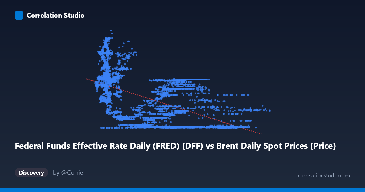
Federal Funds Effective Rate Daily (FRED) (DFF) vs Brent Daily Spot Prices (Price)
- Pearson correlation (r)
- -0.5438
- Spearman correlation
- -0.5951
- p-value
- 0
- Sample size (n)
- 9893
- 95% confidence interval
- -0.5576 to -0.5298
- Granger causality
- None
- Granger optimal lag
- 1
AI analysis
Federal Funds Rate vs. Brent Crude Oil Price: Correlation Analysis
Overview of the Relationship
The scatterplot reveals a negative, moderately dispersed relationship between the Federal Funds Effective Rate (X-axis) and Brent Crude Oil spot prices (Y-axis). The linear regression equation (y = -0.04485x + 5.526) captures a downward trend: as interest rates rise, oil prices tend to be lower on average. However, the visual spread of points is substantial, with oil prices ranging from near zero to nearly $11 (likely in normalized or transformed units) across all rate levels. The data spans nearly four decades (1987–2026), meaning this relationship encapsulates multiple distinct macroeconomic regimes — the 1990s low-rate era, the 2000s commodity boom, the post-2008 zero lower bound period, and the post-2022 rate hiking cycle — each with very different dynamics between monetary policy and energy markets.
Correlation Strength, Direction, and Statistical Significance
The Pearson correlation of r = -0.5438 indicates a moderate negative association, and the R² of 0.2958 means that roughly 29.6% of the variance in oil prices is explained by the federal funds rate — leaving over 70% attributable to other factors entirely. The 95% confidence interval of [-0.5576, -0.5298] is narrow and does not cross zero, and the p-value is effectively 0 across a sample of 9,893 paired observations, making this correlation highly statistically significant. That said, statistical significance here is largely a function of the enormous sample size; a moderate r of -0.54 should not be conflated with strong predictive power. Critically, the Granger causality tests yield no significant directional relationship in either direction (X→Y: F = 0.976, p = 0.323; Y→X: F = 0.115, p = 0.734). This means that at a one-period lag, neither variable reliably predicts the other temporally — the observed correlation is associative, not predictive in the Granger sense, and should not be interpreted as evidence of a causal mechanism operating at daily frequencies.
Notable Patterns, Clusters, and Non-Linear Features
The sample points reveal clear non-linearity and clustering that the linear model cannot fully capture. At very low interest rate levels (X < 30), oil prices span the entire Y range from near zero to ~9, suggesting enormous variance in oil prices during low-rate environments. Conversely, at higher rate levels (X 60–70), nearly all sampled oil prices cluster tightly near zero (e.g., (79.45, 0.20), (82.37, 0.20), (110.05, 0.17), (97.44, 0.08)), suggesting that high interest rate periods historically coincided with depressed oil prices. This asymmetry hints at a possible threshold or hyperbolic decay relationship rather than a simple linear one. The cluster of points at moderate X values (30–55) shows the widest vertical spread, consistent with the 2000s–2010s period of moderate rates and highly volatile oil prices driven by geopolitical and demand shocks.
Confounding Factors and Interpretive Caveats
Several important confounders undermine a causal or even stable interpretation of this correlation. First, reverse causality is plausible: the Fed often raises rates in response to inflationary pressures, some of which are driven by energy price spikes — yet the data show high rates coinciding with low oil prices, suggesting the relationship may be dominated by timing lags across multi-year cycles rather than contemporaneous effects. Second, global supply shocks (OPEC production decisions, the 2014–2016 oil glut, COVID-19 demand collapse) independently drive oil prices regardless of U.S. monetary policy. Third, the U.S. dollar's value — itself influenced by Fed policy — affects oil prices inversely since crude is dollar-denominated, creating an indirect and potentially non-stationary channel. Fourth, the 1987–2026 window encompasses structural breaks (zero lower bound era, shale revolution, energy transition), meaning the correlation likely varies substantially by sub-period and treating it as a single stable relationship is misleading.
Actionable Insights and Further Investigation
Given the moderate correlation, lack of Granger causality, and evident non-linearity, several analytical directions are warranted. Regime-specific analysis — segmenting the data into pre-2008, 2008–2015, 2015–2022, and 2022–present sub-periods — would reveal whether the negative correlation holds consistently or is driven by specific macroeconomic episodes. Non-linear modeling (e.g., polynomial regression, spline fits, or a log transformation of oil prices) would likely improve fit substantially given the visible hyperbolic decay pattern at high rate values. Incorporating control variables such as the U.S. Dollar Index (DXY), global GDP growth proxies, and OPEC production data via multivariate regression would help isolate the independent contribution of interest rates. Finally, extending the Granger causality test to longer lags (3–12 months) may uncover delayed policy transmission effects that are invisible at the one-day lag tested here, and a cointegration analysis (e.g., Johansen test) could assess whether a long-run equilibrium relationship exists between these two series despite the absence of short-run Granger causality.
X dataset: Brent Daily Spot Prices
Y dataset: Federal Funds Effective Rate Daily (FRED)
Part of experiment: Daily - Brent Daily Spot Prices vs Federal Funds Effective Rate Daily (FRED)