Bitcoin Historical Data (2010-2024) (SplyCur) vs Bitcoin Historical Price USD – All-Time Series (Habrador) (Price)
- Pearson correlation (r)
- 0.6144
- Spearman correlation
- 0.9425
- p-value
- 0
- Sample size (n)
- 303
- 95% confidence interval
- 0.539 to 0.68
- Granger causality
- None
- Granger optimal lag
- 10
- Time coverage
- 2010-07-18 to 2011-05-16
- Recomputed on refreshed data
- 2026-10-24 (r was 0.6144)
AI analysis
Analysis: Bitcoin Circulating Supply vs. Price (2010–2011)
1. What the Visualization Reveals
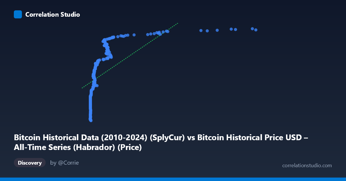
This scatterplot examines the relationship between Bitcoin's circulating supply ("SplyCur") and its historical USD price during a very early window of Bitcoin's existence (July 2010–May 2011). Because supply grows monotonically over time due to the fixed block-reward emission schedule, the X-axis is effectively a proxy for time itself during this period. The data show a clear positive association: as circulating supply increased from roughly 0.05 to 8.2 (units likely in millions of BTC), price climbed from under $3.5M to over $6.2M on whatever normalized/indexed scale this dataset uses. However, the relationship is visibly not a clean straight line — most of the low-supply points are compressed near X≈0.06–0.3, while price at those points varies enormously (from ~3.5M to ~5.3M), indicating a steep, non-linear response at low supply values.
2. Strength, Direction, and Statistical Meaning
The Pearson correlation (r = 0.614) indicates a moderate-to-strong positive linear relationship, with r² = 0.378 meaning the linear model explains only about 38% of the variance in price — leaving nearly two-thirds unexplained by supply alone. The 95% CI [0.539, 0.680] is reasonably tight and excludes zero, and the p-value of ~0 confirms this correlation is highly unlikely to be due to chance. However, statistical significance here reflects the large, non-independent time-series sample rather than necessarily a strong causal signal. Critically, the Granger causality tests show no significant predictive direction in either direction (supply→price: p=0.173; price→supply: p=0.235), meaning that neither variable's history reliably improves forecasts of the other beyond what each series' own past provides. This is an important caveat: correlation exists in level, but there is no evidence of one variable temporally "driving" the other in a predictive sense — consistent with both being driven by a shared underlying process (time/protocol emission) rather than a direct causal supply→price mechanism.
3. Notable Patterns and Non-Linearity
The most striking feature is the clustering of points at very low X values (X < 0.3) where price still spans a wide range ($3.5M–$5.3M), suggesting an early, volatile phase where price was driven by factors other than supply (early speculative trading, low liquidity, exchange listings). Above X≈0.8, points shift to a higher price plateau (~$5.5M–$6.2M) with less spread, suggesting a "step-like" or logarithmic curve rather than a straight line. The note that Spearman's ρ exceeds Pearson's r supports this: the relationship is monotonic but likely curved (concave), fitting better with a logarithmic or power-law model — consistent with the idea that supply increases (roughly linearly with time) while price growth was likely exponential/logarithmic during Bitcoin's early speculative bubble phases.
4. Confounding Factors and Caveats
The dominant confound is time: supply increases mechanically and deterministically via the Bitcoin protocol, so any variable that also trends over time (like early-stage speculative price appreciation) will spuriously correlate with supply. This is a classic case of two non-stationary trending time series producing an inflated correlation without genuine causal linkage — the Granger non-causality result reinforces this interpretation. Additionally, this is a narrow ~10-month window from Bitcoin's earliest history, a period of extreme illiquidity, thin trading volume, and exchange immaturity (e.g., Mt. Gox dominance), making price highly susceptible to idiosyncratic shocks unrelated to supply mechanics.
5. Suggestions for Further Investigation
Given the likely non-linear, time-confounded relationship, analysts should (a) refit using log-price or log-supply transformations, or a polynomial model, to better capture the curvature suggested by the Spearman/Pearson discrepancy; (b) explicitly control for or detrend time to isolate any residual supply-price relationship; (c) test stationarity (e.g., ADF test) before trusting Granger causality results, since non-stationary series can produce misleading causality inference; and (d) extend the analysis across Bitcoin's full 2010–2024 history to see whether the supply-price relationship holds, weakens, or reverses once supply growth decelerates post-halving events, which would better distinguish genuine economic effects (e.g., stock-to-flow dynamics) from early-stage noise.
X dataset: Bitcoin Historical Price USD – All-Time Series (Habrador)
Y dataset: Bitcoin Historical Data (2010-2024)
Part of experiment: Bitcoin - Bitcoin Historical Price USD – All-Time Series (Habrador) vs Bitcoin Historical Data (2010-2024)