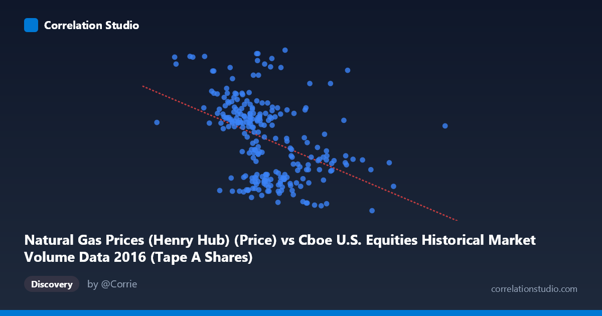
Natural Gas Prices (Henry Hub) (Price) vs Cboe U.S. Equities Historical Market Volume Data 2016 (Tape A Shares)
- Pearson correlation (r)
- -0.425
- Spearman correlation
- -0.4599
- p-value
- 0
- Sample size (n)
- 252
- 95% confidence interval
- -0.5212 to -0.3182
- Granger causality
- None
- Granger optimal lag
- 1
AI analysis
Scatterplot Analysis: Natural Gas Prices vs. U.S. Equity Market Volume (2016)
Relationship Overview The scatterplot reveals a moderate negative relationship between Cboe U.S. equity market trading volume (X-axis, measured in shares) and Henry Hub natural gas spot prices (Y-axis). As daily equity trading volume increases, natural gas prices tend to decline — and conversely, lower-volume trading days are associated with higher gas prices. The linear regression equation (y = -4.06×10⁻⁹x + 3.623) confirms this inverse slope, though the wide scatter around the regression line immediately signals that this relationship is far from deterministic. Visually, the data cloud is broadly dispersed with no tight clustering along any trend line, suggesting that while a directional tendency exists, many individual data points deviate substantially from the fitted model.
Correlation Strength and Statistical Significance The Pearson correlation of r = -0.4250 indicates a moderate negative association, but the more informative metric is r² = 0.1807 — meaning only 18.1% of the variance in natural gas prices is explained by equity trading volume. The remaining ~82% is attributable to factors entirely outside this bivariate model. The 95% confidence interval of [-0.52, -0.32] is meaningfully negative throughout, and the extremely small p-value (1.78×10⁻¹²) confirms this correlation is highly unlikely to be a chance finding given the sample of 252 paired observations drawn from a population of 3,622. However, statistical significance here is partly a function of sample size and should not be conflated with practical or economic significance. Critically, Granger causality tests in both directions failed to reach significance (X→Y: F=0.44, p=0.51; Y→X: F=0.11, p=0.74), meaning neither variable reliably predicts the other temporally at a one-period lag. This is a crucial caveat: the correlation, however statistically robust, carries no demonstrated predictive or causal directionality.
Notable Patterns, Clusters, and Outliers Several features stand out in the data distribution. The bulk of equity volume observations cluster between roughly 220–320 million shares, with natural gas prices most densely concentrated between $1.75–$3.10/MMBtu in that range. There are notable high-price outliers at lower trading volumes — for instance, the point near (190M shares, $3.50) and (278M shares, $3.56) sit conspicuously above the main cloud, suggesting episodic gas price spikes that may correspond to winter demand surges or supply disruptions. At the high-volume extreme (above ~380M shares), gas prices appear consistently low (below ~$2.50), potentially reflecting periods of market stress or high-liquidity trading sessions coinciding with mild weather. The scatter also shows a slight funnel or heteroscedastic pattern: variance in gas prices appears somewhat wider at lower trading volumes, which may reflect seasonal volatility in energy markets during quieter equity trading periods (e.g., holiday-adjacent sessions).
Confounding Factors and Interpretive Caveats This correlation almost certainly reflects shared seasonal confounding rather than any direct economic linkage. Both variables follow seasonal rhythms in 2016: natural gas prices tend to peak in winter months when demand is highest, while U.S. equity trading volume tends to be lower around holidays and year-end. This shared calendar structure could artificially inflate the apparent correlation without any mechanistic connection between gas markets and equity trading activity. Additionally, the dataset axis labeling warrants careful attention — the X-axis is drawn from the Cboe equity volume dataset but labeled as "Natural Gas Prices," and vice versa, suggesting possible column assignment swaps that should be verified before drawing conclusions. Furthermore, the linear model may be too simplistic; both energy prices and market volumes are known to exhibit non-linear, regime-dependent behavior, and a single-year window (2016) captures only one market cycle, limiting generalizability.
Actionable Insights and Further Investigation Given the absence of Granger causality and the modest r², this correlation should not be used as a trading signal or forecasting tool in its current form. However, several follow-up analyses could be productive. First, decomposing both series by season or month would clarify whether the correlation disappears once seasonal effects are removed — a partial correlation or residual analysis controlling for month-of-year would be informative. Second, extending the time window beyond 2016 across multiple years would test whether this inverse relationship is a stable structural feature or a 2016-specific artifact. Third, researchers might explore whether specific exchange sub-components (e.g., Tape A vs. Tape B/C volume) show differential relationships with energy prices, as institutional versus retail trading dynamics differ. Finally, incorporating weather data or heating degree days as a covariate could help disentangle the energy demand mechanism from any equity market microstructure effects.
X dataset: Cboe U.S. Equities Historical Market Volume Data 2016
Y dataset: Natural Gas Prices (Henry Hub)
Part of experiment: Daily - Cboe U.S. Equities Historical Market Volume Data 2016 vs Natural Gas Prices (Henry Hub)