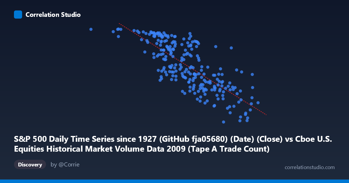
S&P 500 Daily Time Series since 1927 (GitHub fja05680) (Date) (Close) vs Cboe U.S. Equities Historical Market Volume Data 2009 (Tape A Trade Count)

Pearson correlation (r): -0.7756
Spearman correlation: -0.7856
p-value: 0
Sample size (n): 252
95% confidence interval: -0.8206 to -0.7212
Granger causality: X → Y
Granger optimal lag: 10

AI analysis

Analysis: S&P 500 Price Level vs. Cboe Tape A Trade Count (2009)

Relationship Overview The scatterplot reveals a clear negative relationship between the S&P 500 closing price (X-axis) and Cboe Tape A trade count (Y-axis) across 252 trading days in 2009. As the S&P 500 price level rises, the number of individual trades executed on Tape A venues declines meaningfully. This pattern is economically intuitive given the temporal context: 2009 began near the nadir of the Global Financial Crisis, when prices were depressed but market activity (particularly retail panic selling and institutional repositioning) was frantic. As markets recovered through the year, elevated speculative trading gradually subsided, producing the observed inverse arc.

Correlation Strength and Statistical Robustness The Pearson correlation of r = −0.776 is strong and negative, with the linear regression slope of approximately −0.000230 trades per index point confirming the direction. Critically, R² = 0.602 means that roughly 60% of the variance in trade count is explained by the S&P 500 price level alone — a substantial but incomplete explanation, leaving 40% attributable to other factors. The 95% confidence interval of [−0.821, −0.721] is narrow and entirely negative, indicating high confidence in the direction and approximate magnitude of the relationship. The p-value of essentially zero eliminates any concern about chance findings at this sample size (n = 252). The Granger causality result adds a directionally important nuance: X unidirectionally Granger-causes Y at an optimal lag of 10 trading periods (F = 1.97, p = 0.038), while Y does not Granger-cause X (p = 0.126). This means S&P 500 price movements have statistically significant predictive power over future trade counts approximately two weeks ahead, but trade volume activity does not similarly predict future price levels in this dataset — suggesting price leads behavioral trading activity rather than the reverse.

Notable Patterns, Clusters, and Outliers The data form a broad but coherent downward-sloping cloud with several notable features. There is a distinct high-trade-count cluster at low price levels (roughly X < 900,000–1,100,000 range mapped to early 2009 crisis lows), where trade counts consistently approach or exceed 1,050–1,127. Conversely, as prices push above ~2,000,000–2,500,000 in the index's scaled representation, trade counts compress into the 683–770 range. The point (362,081; 1,126) stands out as a potential early-year extreme outlier with the lowest price and near-maximum trade count, consistent with early January 2009 crisis conditions. Several points in the upper-right quadrant (e.g., ~2,549,192; 770 and ~2,405,270; 683) represent late-year high-price/low-activity sessions. The scatter is notably heteroscedastic — variance in trade counts is wider at lower price levels than at higher ones, suggesting that fear-driven markets produce more erratic trading behavior than calmer recovery-phase markets.

Confounding Factors and Interpretive Caveats Several important caveats apply. First, this correlation is fundamentally temporal in nature — both variables are trending across a single calendar year (prices rising from crisis lows, trading frenzy subsiding), so the relationship may largely reflect shared time-series trends rather than a direct causal mechanism. This is a classic spurious correlation risk driven by common temporal evolution. Second, market structure changes in 2009 (e.g., algorithmic trading growth, exchange fee adjustments, regulatory responses to the crisis) could independently affect trade counts regardless of price level. Third, Tape A specifically covers NYSE-listed securities; shifts in exchange market share throughout 2009 could distort trade count trends. Fourth, the 10-period Granger lag (~2 calendar weeks) is suggestive but relatively modest in predictive F-statistic (1.97), meaning the practical forecasting edge is real but not overwhelming. Finally, with N = 3,232 as the population size versus n = 252 sampled, the sample appears to be every trading day — so sampling bias is minimal, but generalizability beyond 2009 crisis conditions should not be assumed.

Actionable Insights and Further Investigation Practitioners and researchers should consider several follow-up analyses. Detrending both series (e.g., first-differencing or regressing out the time trend) would test whether the relationship holds beyond shared temporal drift — a critical validity check before drawing structural conclusions. The 10-period Granger lag warrants practical exploration: a trader or risk manager could test whether S&P 500 price momentum over a two-week window provides actionable forecasts of near-term trading activity and liquidity conditions. Extending the analysis to multiple years (particularly comparing crisis vs. non-crisis years) would reveal whether this inverse relationship is a 2009-specific crisis artifact or a more durable market microstructure pattern. Additionally, decomposing trade count by investor type (retail vs. institutional) or by volatility regime (using VIX as a covariate) would likely absorb much of the unexplained 40% variance and clarify the behavioral mechanism driving elevated trading at depressed price levels.

X dataset: Cboe U.S. Equities Historical Market Volume Data 2009

Y dataset: S&P 500 Daily Time Series since 1927 (GitHub fja05680) (Date)

Part of experiment: Daily - Cboe U.S. Equities Historical Market Volume Data 2009 vs S&P 500 Daily Time Series since 1927 (GitHub fja05680) (Date)