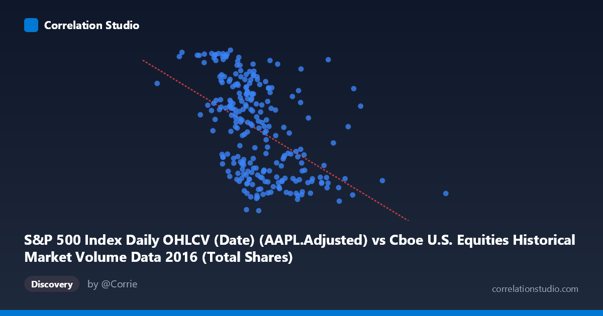
S&P 500 Index Daily OHLCV (Date) (AAPL.Adjusted) vs Cboe U.S. Equities Historical Market Volume Data 2016 (Total Shares)
- Pearson correlation (r)
- -0.4785
- Spearman correlation
- -0.5175
- p-value
- 0
- Sample size (n)
- 252
- 95% confidence interval
- -0.5684 to -0.3772
- Granger causality
- None
- Granger optimal lag
- 1
AI analysis
Scatterplot Analysis: AAPL Adjusted Price vs. Cboe Total Shares Volume (2016)
1. Overall Relationship The scatterplot reveals a moderate negative relationship between Apple's adjusted stock price (X-axis) and total U.S. equity shares traded on Cboe exchanges (Y-axis) across 252 trading days in 2016. As AAPL's adjusted price increases, total market share volume tends to decline, and vice versa. The linear regression equation (y = -3.43×10⁻⁸x + 120.725) confirms this inverse slope, with the fitted line descending from left to right across the plot. However, substantial vertical scatter around the regression line is immediately evident, suggesting the relationship is real but far from deterministic.
2. Correlation Strength, Direction, and Causality The Pearson correlation of r = -0.4785 indicates a moderate negative association — statistically meaningful but not dominant. Critically, the R² of 0.2289 means only ~22.9% of the variance in total share volume is explained by AAPL's adjusted price, leaving roughly 77% attributable to other factors. The 95% confidence interval of [-0.5684, -0.3772] is entirely negative and does not cross zero, reinforcing directional confidence. The p-value of 8.88×10⁻¹⁶ is astronomically small, confirming the correlation is highly unlikely to be a chance artifact given n = 252. Despite statistical significance, the Granger causality tests reveal no meaningful temporal predictive relationship in either direction (X→Y: F = 0.552, p = 0.458; Y→X: F = 1.322, p = 0.251). This is a crucial caveat: knowing today's AAPL price does not help predict tomorrow's market volume, and vice versa — the correlation appears contemporaneous rather than predictively directional.
3. Notable Patterns, Clusters, and Outliers Several features stand out in the sample data. The bulk of observations cluster between AAPL prices of ~$420M–$570M and volumes of ~90–115 total shares, forming a loose but discernible downward-sloping cloud. There are visible outliers at both extremes: one point near X ≈ 708M with Y ≈ 93.8, and another near X ≈ 369M with Y ≈ 116.6, both consistent with the inverse trend but sitting far from the central cluster. The Y range is notably compressed (89.01–117.14, stdev ~8), while X spans a much wider proportional range (~200M–1.09B, stdev ~111M), suggesting volume is relatively stable while price varies more dramatically. Some vertical banding is visible, hinting at possible discretization or periodic reporting in the volume data.
4. Confounding Factors and Caveats This correlation almost certainly reflects shared macroeconomic seasonality rather than a direct causal mechanism. AAPL prices were generally lower in early 2016 during a market downturn and recovered later in the year, while overall market volume tends to be higher during volatile, uncertain periods (which coincide with lower prices). This creates a spurious inverse correlation driven by a common underlying factor: market volatility or risk sentiment. Additionally, the axes appear to be swapped from their conventional roles — the dataset labels suggest AAPL Adjusted Price is on the X-axis but sourced from the Cboe volume dataset, and vice versa, which warrants verification. The n = 252 paired sample drawn from N = 506 may also introduce selection bias depending on how pairs were matched.
5. Actionable Insights and Further Investigation Given the lack of Granger causality, practitioners should avoid using this relationship for short-term predictive trading signals. Instead, the correlation is better interpreted as a risk regime indicator — periods of elevated AAPL prices may coincide with calmer, lower-volume markets. Suggested next steps include: (1) incorporating VIX or implied volatility as a control variable to test whether it mediates or eliminates this correlation; (2) segmenting by calendar quarter to test whether the relationship holds uniformly or is driven by specific periods (e.g., Q1 2016 selloff); (3) testing non-linear models (e.g., quadratic or spline regression) given the visible scatter heterogeneity; and (4) verifying axis/dataset assignments to ensure the variable roles are correctly interpreted before drawing any investment conclusions.
X dataset: Cboe U.S. Equities Historical Market Volume Data 2016
Y dataset: S&P 500 Index Daily OHLCV (Date)
Part of experiment: Daily - Cboe U.S. Equities Historical Market Volume Data 2016 vs S&P 500 Index Daily OHLCV (Date)