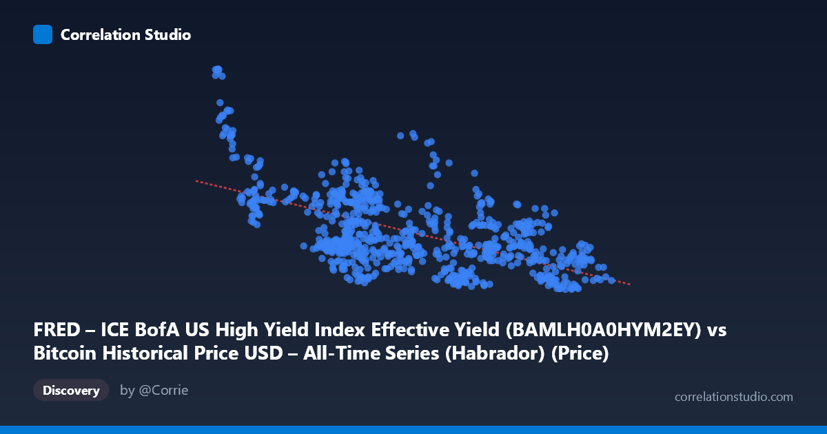
FRED – ICE BofA US High Yield Index Effective Yield (BAMLH0A0HYM2EY) vs Bitcoin Historical Price USD – All-Time Series (Habrador) (Price)
- Pearson correlation (r)
- -0.6566
- Spearman correlation
- -0.6122
- p-value
- 0
- Sample size (n)
- 668
- 95% confidence interval
- -0.6977 to -0.6112
- Granger causality
- None
- Granger optimal lag
- 1
AI analysis
Analysis: Bitcoin Price vs. High Yield Bond Effective Yield
1. Overview of the Relationship
The scatterplot displays a clear negative relationship between Bitcoin's price (X-axis, ranging from ~$25K to ~$125K) and the ICE BofA US High Yield Index Effective Yield (Y-axis, ranging from 6.39% to 9.45%). As Bitcoin's price rises, the high-yield bond effective yield tends to fall, and vice versa. This pattern is visually consistent: low Bitcoin prices (sub-$35K) cluster with high yields (8-9.5%), while high Bitcoin prices (above $90K) cluster with lower, compressed yields (6.5-7.5%).
2. Strength, Direction, and Statistical Confidence
The correlation coefficient of r = -0.7702 indicates a strong negative linear relationship. The r² = 0.5932 means approximately 59% of the variance in high-yield bond yields can be statistically associated with Bitcoin price movements — a substantial but not overwhelming share, leaving 41% of variance driven by other factors. The tight 95% confidence interval [-0.7975, -0.7397] and a p-value of 0 (effectively zero, given n=765) confirm this correlation is highly statistically significant and not a product of sampling noise. However, the Granger causality tests are critical here: neither direction shows significance (X→Y: p=0.47; Y→X: p=0.37). This means neither variable reliably predicts future movements in the other based on past values. The relationship appears to be a strong contemporaneous/structural association rather than a causal, time-lagged predictive one — both variables likely respond to a shared underlying driver (e.g., macro risk sentiment, Fed policy) rather than one leading the other.
3. Patterns and Notable Features
The data shows a discernible non-linear, curved pattern rather than a purely linear one — yields drop steeply as Bitcoin rises from $25K to $60K, then flatten into a tighter band (6.5-7.5%) as Bitcoin exceeds $90K, suggesting diminishing sensitivity at higher price levels (possible saturation or floor effect in yields). There's also noticeable vertical scatter at the high end (e.g., prices near $90-95K showing yields from 6.43 to 7.75), indicating that other factors introduce noise once Bitcoin prices are elevated. No extreme outliers are evident from the sample; the relationship appears reasonably continuous across the range.
4. Confounding Factors and Caveats
Both series are likely driven by shared macroeconomic conditions — risk appetite, Fed monetary policy, inflation expectations, and liquidity conditions can simultaneously suppress bond yields (via flight-to-quality reversals or rate-cut expectations) and boost speculative assets like Bitcoin. This makes the relationship likely spurious in a causal sense, reflecting correlation through a common macro factor rather than a direct economic link between crypto and junk bonds. Additionally, both are time series with trends, and non-stationarity can inflate correlation estimates (a classic issue when two trending series are compared without differencing/detrending). The 2023-2026 window also coincides with a specific monetary cycle (likely rate cuts/easing), which may not generalize to other regimes.
5. Suggested Next Steps
To move beyond this descriptive correlation: (1) test both series for stationarity (ADF test) and consider correlating returns/differences rather than levels to avoid spurious trend-driven correlation; (2) incorporate a common macro variable (e.g., Fed funds rate, VIX, or 10Y Treasury yield) as a control in a multivariate regression to test if the BTC-HY relationship holds after controlling for shared drivers; (3) given the non-linear flattening pattern, test a log or polynomial fit which may improve explanatory power beyond the current linear R²=0.593; (4) since Granger causality is absent, avoid using either series as a leading indicator for the other in trading/forecasting models — treat this as a coincident risk-sentiment relationship rather than predictive signal.
X dataset: Bitcoin Historical Price USD – All-Time Series (Habrador)
Y dataset: FRED – ICE BofA US High Yield Index Effective Yield
Part of experiment: Bitcoin - Bitcoin Historical Price USD – All-Time Series (Habrador) vs FRED – ICE BofA US High Yield Index Effective Yield