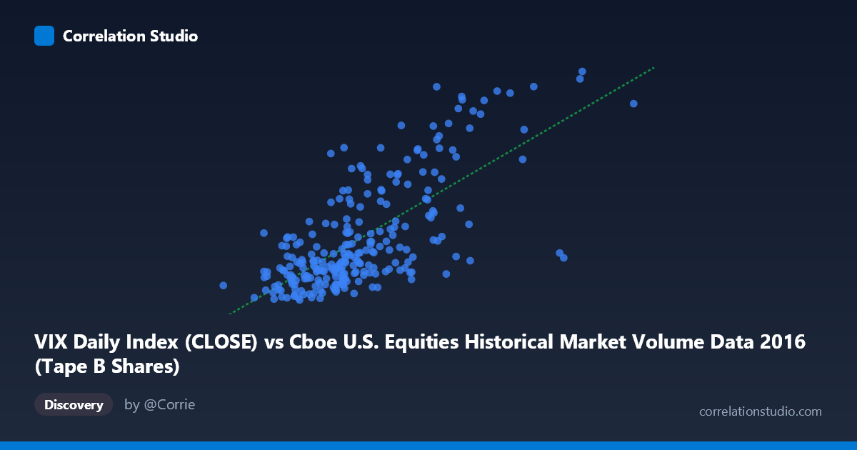
VIX Daily Index (CLOSE) vs Cboe U.S. Equities Historical Market Volume Data 2016 (Tape B Shares)

Pearson correlation (r): 0.7051
Spearman correlation: 0.6568
p-value: 0
Sample size (n): 252
95% confidence interval: 0.6371 to 0.7623
Granger causality: None
Granger optimal lag: 1

AI analysis

Scatterplot Analysis: VIX Daily Index vs. Tape B Shares (2016)

Relationship Overview The scatterplot reveals a moderate-to-strong positive relationship between the CBOE Volatility Index (VIX) closing values and Tape B share volumes in U.S. equity markets during 2016. As VIX levels rise — indicating greater market uncertainty and fear — Tape B trading volumes tend to increase correspondingly. The linear regression equation (y = 9.25×10⁻⁸x + 5.91) captures this upward trend, and the scatter of points broadly follows this trajectory, though with considerable dispersion around the fitted line. This pattern is consistent with well-established market microstructure theory: elevated volatility typically drives heightened trading activity as investors reposition, hedge, or react to rapidly changing price signals.

Correlation Strength and Statistical Significance The Pearson correlation of r = 0.705 indicates a moderately strong positive association, but the more instructive figure is r² = 0.497 — meaning approximately 49.7% of the variance in Tape B share volume is explained by VIX levels. While meaningful, this also implies that roughly half of the variation in trading volume is attributable to other factors entirely. The 95% confidence interval of [0.637, 0.762] is relatively tight and excludes zero, and the p-value of effectively 0 confirms the result is highly statistically significant across the full population of N = 3,622 observations. However, the Granger causality tests reveal no significant temporal predictive relationship in either direction (X→Y: F = 0.157, p = 0.692; Y→X: F = 0.072, p = 0.788). This is a critical caveat: despite the strong contemporaneous correlation, neither variable reliably predicts the other at a one-period lag, suggesting the relationship is largely concurrent rather than directionally causal at the daily frequency examined.

Notable Patterns, Clusters, and Outliers The sample points reveal several visually distinct features. The bulk of observations cluster in the lower-left region — VIX values roughly between 75M–105M and Tape B shares between 12 and 16 — suggesting that calm, low-volatility days dominate the 2016 trading calendar. However, a notable upper-right cluster of high-leverage outliers is visible, including points such as (170.6M, 26.69) and (126.1M, 24.15), which correspond to periods of acute market stress (likely around the Brexit vote in June and post-U.S. election volatility in November 2016). These extreme observations exert disproportionate influence on the correlation coefficient and may be inflating the apparent strength of the linear relationship. The dispersion also appears to fan outward at higher VIX values, hinting at possible heteroscedasticity — variance in volume increases as volatility rises, which violates a core assumption of ordinary least squares regression.

Confounding Factors and Interpretive Caveats Several important confounds merit attention. First, calendar effects such as end-of-quarter rebalancing, option expiration dates, and holiday-adjacent low-volume days can simultaneously depress VIX and suppress volumes, creating spurious co-movement. Second, structural market events in 2016 — Brexit (June 23), the U.S. presidential election (November 8), and Federal Reserve policy decisions — represent discrete regime shifts that could drive both variables upward simultaneously without implying a stable underlying mechanism. Third, the axis labeling appears transposed relative to conventional interpretation: the dataset notes indicate VIX is on the X-axis while Tape B Shares (from the VIX dataset) are on the Y-axis, which warrants verification to ensure the regression direction is analytically meaningful. Finally, Tape B specifically covers NYSE American (AMEX) and regional exchange securities, so volume dynamics here may not generalize to broader market behavior captured by Tape A or C.

Actionable Insights and Further Investigation Practitioners and researchers should consider several follow-up steps. Given the heteroscedasticity concern, applying a log-log transformation to both variables may stabilize variance and yield a more robust regression fit. The absence of Granger causality at lag 1 is worth extending — testing longer lag structures (2–5 days) could reveal delayed transmission effects that are economically meaningful for trading strategy design. It would also be valuable to segment the analysis by volatility regime (e.g., VIX < 15 vs. VIX 20) to determine whether the correlation holds uniformly or is driven almost entirely by stress episodes. Finally, incorporating additional explanatory variables — such as options expiration indicators, Fed announcement days, or cross-asset flow measures — into a multivariate framework could help explain the remaining ~50% of variance and build a more actionable predictive model for volume forecasting.

X dataset: Cboe U.S. Equities Historical Market Volume Data 2016

Y dataset: VIX Daily Index

Part of experiment: Daily - Cboe U.S. Equities Historical Market Volume Data 2016 vs VIX Daily Index