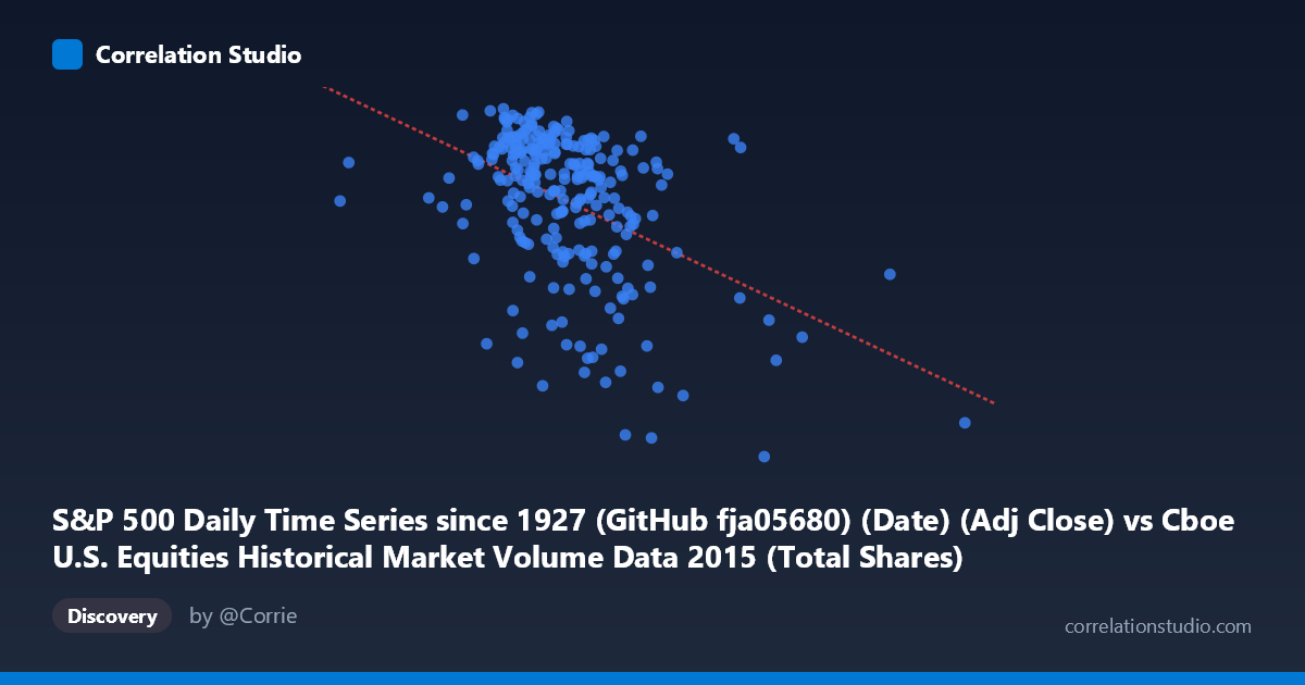
S&P 500 Daily Time Series since 1927 (GitHub fja05680) (Date) (Adj Close) vs Cboe U.S. Equities Historical Market Volume Data 2015 (Total Shares)

Pearson correlation (r): -0.4486
Spearman correlation: -0.4142
p-value: 0
Sample size (n): 252
95% confidence interval: -0.5421 to -0.3441
Granger causality: X → Y
Granger optimal lag: 5

AI analysis

S&P 500 Price vs. U.S. Equity Market Trading Volume (2015)

Relationship Overview The scatterplot reveals a moderate negative relationship between U.S. equity market total shares traded (X-axis) and the S&P 500 adjusted closing price (Y-axis) across 2015 trading days. As daily trading volume increases, the S&P 500 price level tends to decline — a counterintuitive but well-documented market dynamic. The linear regression equation (y = -2.53×10⁻⁷x + 2194.35) confirms this inverse slope, meaning that for every additional ~4 billion shares traded in a day, the S&P 500 tends to be approximately 1 point lower. The relationship is visually discernible but far from deterministic, with considerable scatter throughout the plot, particularly in the mid-range volume zone.

Correlation Strength and Statistical Significance The Pearson correlation of r = -0.4486 indicates a moderate negative association, but the coefficient of determination tells a more sobering story: r² = 0.2012 means that only ~20% of the day-to-day variance in S&P 500 price levels is explained by total shares traded, leaving roughly 80% attributable to other factors. The 95% confidence interval of [-0.5421, -0.3441] is meaningfully narrow and does not cross zero, and the p-value of 7.0×10⁻¹⁴ confirms this relationship is statistically significant well beyond conventional thresholds — effectively eliminating chance as an explanation given n = 252. Critically, the Granger causality analysis identifies a unidirectional predictive relationship: X Granger-causes Y (F = 2.34, p = 0.0425) with an optimal lag of 5 trading days, while the reverse direction fails to achieve significance (F = 0.37, p = 0.871). This suggests that elevated trading volume today may have modest predictive value for S&P 500 price levels approximately one week later, though the F-statistic is modest and the relationship should not be over-interpreted as causal.

Notable Patterns, Clusters, and Outliers Several structural features are visible in the data. The bulk of observations cluster in the 400–650 million share range with S&P prices between approximately 2,040–2,130, forming a relatively dense core that anchors the regression line. However, there is a distinct lower-right cluster of high-volume, low-price observations — points exceeding 650–800 million shares traded with S&P values in the 1,870–1,990 range — that disproportionately drives the negative slope. These points likely correspond to the August–September 2015 market selloff, when extreme volatility triggered panic selling and sharp price declines alongside historically elevated volume. At least two points near 808–815 million shares with prices around 1,868–1,971 appear as potential outliers and warrant individual examination. Meanwhile, the upper-left of the plot shows high S&P prices (2,120–2,130) concentrated at moderate-to-lower volumes, consistent with the quieter, low-volatility rally periods earlier in 2015.

Confounding Factors and Interpretive Caveats The most important caveat is that this correlation likely reflects a common response to a third variable — market volatility or fear — rather than a direct mechanistic link between volume and price. During stress events, both price declines and volume spikes are simultaneously driven by investor sentiment, institutional de-risking, and margin calls. The relationship may therefore be spurious in a causal sense, with the August 2015 correction functioning as a high-leverage event that inflates the apparent correlation. Additionally, the data covers only a single calendar year (2015), limiting generalizability; in bull market years with low volatility, the volume-price relationship might be flat or even positive. The Granger test, while suggestive, only demonstrates predictive precedence within this sample — not economic causation — and a lag of 5 periods may be capturing mean-reversion dynamics post-selloff rather than a structural volume-leads-price mechanism.

Actionable Insights and Further Investigation Several lines of follow-up analysis are warranted. First, replicating this analysis across multiple years (e.g., 2010–2023) would test whether the negative relationship is a consistent feature of market structure or an artifact of the 2015 stress period. Second, conditioning the analysis on volatility regime (e.g., using the VIX as a stratifying variable) would help isolate whether the volume-price relationship persists after controlling for fear/uncertainty. Third, the 5-day Granger lag deserves exploration as a potential short-term trading signal — specifically, whether above-threshold volume days reliably predict below-average returns over the following week net of transaction costs. Finally, decomposing total shares into buy-initiated vs. sell-initiated volume (using TAQ or similar data) could reveal whether it is selling pressure specifically — rather than total activity — that carries the predictive content suggested by the Granger result.

X dataset: Cboe U.S. Equities Historical Market Volume Data 2015

Y dataset: S&P 500 Daily Time Series since 1927 (GitHub fja05680) (Date)

Part of experiment: Daily - Cboe U.S. Equities Historical Market Volume Data 2015 vs S&P 500 Daily Time Series since 1927 (GitHub fja05680) (Date)