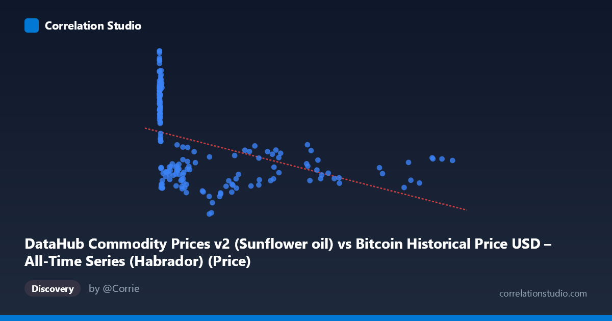
DataHub Commodity Prices v2 (Sunflower oil) vs Bitcoin Historical Price USD – All-Time Series (Habrador) (Price)
- Pearson correlation (r)
- -0.4319
- Spearman correlation
- -0.6898
- p-value
- 0
- Sample size (n)
- 182
- 95% confidence interval
- -0.5433 to -0.3057
- Granger causality
- None
- Granger optimal lag
- 9
- Time coverage
- 2010-08-01 to 2025-09-01
- Recomputed on refreshed data
- 2026-10-24 (r was -0.4319)
AI analysis
Analysis: Sunflower Oil Prices vs. Bitcoin Historical Prices
Note on axis labeling: The dataset naming appears swapped based on the note context — this analysis treats X as sunflower oil commodity price and Y as the Bitcoin-associated price series (or vice versa) purely by the statistical relationship shown, since the scatterplot data suggests X spans a huge range (0.06 to 113,500) consistent with Bitcoin's price history from genesis to present, while Y (614–974) behaves more like an index or commodity price scale.
1. What the Visualization Reveals
The scatterplot shows a negative, moderate-strength relationship between the two variables. As X increases, Y tends to decrease, but the relationship is far from clean or deterministic — there's substantial scatter around any fitted line. At very low X values (under ~100), Y clusters tightly in the 820–960 range with high values, while as X grows into the thousands and tens-of-thousands range, Y drops and stabilizes in a lower band (roughly 660–760), with more variance.
2. Strength, Direction, and Statistical Confidence
The Pearson correlation of r = -0.432 indicates a moderate negative linear association. However, r² = 0.187 tells the more important story: only 18.7% of the variance in Y is explained by X. This means over 80% of Y's variability is driven by other factors, noise, or non-linear structure not captured by this simple linear model. The 95% CI [-0.543, -0.306] is reasonably tight and excludes zero, and the p-value (1.14E-09) confirms this correlation is statistically robust — not a fluke of sampling. That said, statistical significance ≠ practical strength: this is a real but weak-to-moderate relationship.
Critically, the Granger causality tests show no significant predictive direction in either direction (X→Y: p=0.70; Y→X: p=0.22). This strongly suggests that despite the contemporaneous correlation, neither variable temporally leads or forecasts the other in a Granger sense. This is an important caveat: the correlation may reflect a shared external driver (e.g., both influenced by macroeconomic conditions, USD strength, time trends, or inflation) rather than any causal or predictive link between the two.
3. Notable Patterns and Outliers
The data show a strong non-linear signature: at low X (near zero), Y values are elevated and tightly clustered (860–960), and as X scales up logarithmically, Y decreases and plateaus. This is a classic log-decay pattern, not a straight line — consistent with the note that Spearman ρ exceeds Pearson r, confirming a monotonic but curved relationship. A log-transform of X would likely fit far better than the current linear model (R²=0.187). There are also outlier-like points at very high X (e.g., 97,365 and 105,620) where Y rebounds upward (689 and 739) rather than continuing to decline, suggesting the relationship may flatten or even reverse at extreme X values — possibly reflecting different market regimes (e.g., late-cycle Bitcoin bull markets).
4. Confounding Factors and Caveats
Both series span 2010–2025, a period marked by major macroeconomic shifts — the pandemic, inflation waves, USD strength cycles, and commodity supply shocks (e.g., sunflower oil disruption from the 2022 Ukraine war). Any correlation between a rapidly-scaling asset price and a commodity price index is highly susceptible to spurious correlation via shared time trends rather than direct economic linkage. Since Bitcoin trades in an entirely different market ecosystem than edible oils, a genuine causal mechanism is implausible — this is far more likely a time-series confound (both trending over the same calendar period) than a meaningful economic relationship.
5. Suggestions for Further Investigation
- Fit a log-linear or log-log model on X to test if it substantially improves R² given the apparent log-decay curve. - Detrend both series (e.g., first-difference or de-mean by year) before correlating, to rule out spurious trend-driven correlation. - Test with lagged cross-correlation at finer granularity than the 9-period Granger lag, since monthly commodity data and Bitcoin's volatility operate on different timescales. - Treat this relationship as descriptive, not predictive or causal — it should not be used for trading signals or forecasting given the null Granger result and modest r².
X dataset: Bitcoin Historical Price USD – All-Time Series (Habrador)
Y dataset: DataHub Commodity Prices v2
Part of experiment: Bitcoin - Bitcoin Historical Price USD – All-Time Series (Habrador) vs DataHub Commodity Prices v2