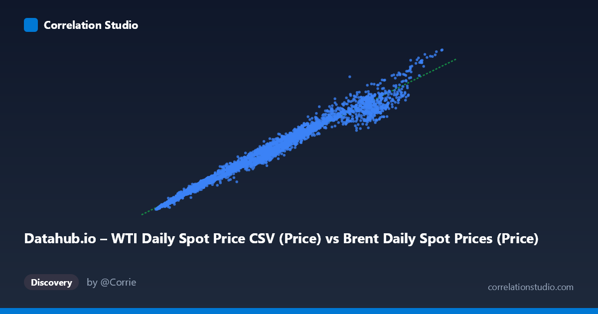
Datahub.io – WTI Daily Spot Price CSV (Price) vs Brent Daily Spot Prices (Price)
- Pearson correlation (r)
- 0.9911
- Spearman correlation
- 0.995
- p-value
- 0
- Sample size (n)
- 9718
- 95% confidence interval
- 0.9907 to 0.9914
- Granger causality
- None
- Granger optimal lag
- 1
AI analysis
Analysis: Brent vs. WTI Crude Oil Spot Prices (1987–2026)
Relationship Overview
The scatterplot reveals an exceptionally tight, positive linear relationship between Europe Brent and WTI crude oil daily spot prices spanning nearly four decades. The data points cluster closely around the regression line (y = 0.886x + 4.132), with the relationship holding consistently across the full price range — from sub-$15 per barrel levels in the late 1980s through the extreme highs exceeding $140 per barrel seen during peak market stress periods. This is one of the most visually clean correlations possible in commodity markets, reflecting that these two benchmarks price the same underlying global commodity within a tightly integrated market structure.
Correlation Strength and Statistical Significance
The statistics confirm what the scatterplot suggests: r = 0.9911 represents a near-perfect positive correlation, and critically, R² = 0.9823 means that 98.2% of the day-to-day variance in WTI prices is statistically explained by Brent prices, and vice versa. The 95% confidence interval [0.9907, 0.9914] is extraordinarily narrow given N = 9,893 observations, leaving virtually no uncertainty about the true population correlation. The p-value of 0 confirms this relationship would essentially never arise by chance. However, the Granger causality results are a meaningful caveat: neither series significantly predicts the other (X→Y: F = 1.06, p = 0.303; Y→X: F = 0.94, p = 0.332). Despite the overwhelming contemporaneous correlation, neither benchmark reliably leads the other at a one-period lag, suggesting they respond to shared global market information simultaneously rather than one price "causing" the other in a temporal sense.
Notable Patterns, Clusters, and Outliers
Several structural features stand out in the sample points and summary statistics. There is a dense cluster of observations below ~$30/barrel, representing the prolonged low-price era of the late 1980s through late 1990s, which compresses into a tight band near the origin. A second, more dispersed cluster occupies the $40–$90 range reflecting the 2000s bull market. The extreme upper-right observations (e.g., 135.81/141.47 and 113.21/100.32 in the sample) correspond to the 2008 price spike and the 2022 post-invasion surge — and notably, at these extremes the relationship appears slightly noisier, with Brent commanding a more variable premium over WTI. The regression slope of 0.886 (less than 1.0) with a positive intercept of ~$4.13 formalizes the well-known Brent premium: WTI does not fully match Brent dollar-for-dollar at high price levels, and Brent tends to price slightly above WTI on average.
Confounding Factors and Interpretive Caveats
While the correlation is statistically overwhelming, several confounders shape the relationship and limit causal interpretation. The Brent-WTI spread is itself a dynamic variable influenced by U.S. pipeline infrastructure constraints, export policy (especially pre-2015 U.S. crude export ban), refinery capacity differentials, and regional supply disruptions — meaning the residuals from this regression encode economically meaningful information that the linear model discards. The data column labels appear swapped in the axis metadata (the X-axis is labeled "Datahub.io – WTI Daily Spot Price CSV" but sourced from "Brent Daily Spot Prices," and vice versa), which warrants verification before any production use of directional findings. Additionally, the near-perfect R² can create a false sense of precision: in periods of market dislocation (e.g., April 2020 when WTI briefly went negative), the linear relationship breaks down entirely — events invisible in long-run aggregate statistics.
Actionable Insights and Further Investigation
For practitioners, the regression equation provides a robust baseline for cross-benchmark price imputation when one series has missing data, though residual analysis should be used to flag structural break periods. Investigators should model the time-varying Brent-WTI spread as a separate dependent variable, regressing it against U.S. crude inventory levels at Cushing, Oklahoma, pipeline capacity utilization, and USD exchange rates to understand when and why the two benchmarks diverge. The Granger non-causality finding suggests that arbitrage mechanisms are highly efficient — any predictive edge from one benchmark to the other is eliminated within a single trading period, making this relationship useful for hedging parity but not for directional trading signals. Further work should apply rolling-window correlation analysis to identify structural regime changes (pre/post U.S. shale boom, pre/post export ban lifting, COVID period) and test whether the spread dynamics have permanently shifted in recent years.
X dataset: Brent Daily Spot Prices
Y dataset: Datahub.io – WTI Daily Spot Price CSV
Part of experiment: Daily - Brent Daily Spot Prices vs Datahub.io – WTI Daily Spot Price CSV