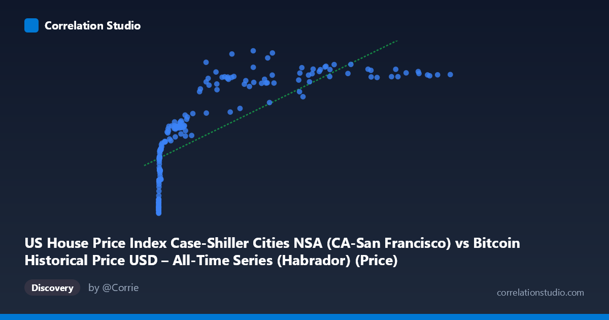
US House Price Index Case-Shiller Cities NSA (CA-San Francisco) vs Bitcoin Historical Price USD – All-Time Series (Habrador) (Price)
- Pearson correlation (r)
- 0.76
- Spearman correlation
- 0.9606
- p-value
- 0
- Sample size (n)
- 191
- 95% confidence interval
- 0.6928 to 0.8141
- Granger causality
- None
- Granger optimal lag
- 10
- Time coverage
- 2010-08-01 to 2026-06-01
- Recomputed on refreshed data
- 2026-10-24 (r was 0.7541)
AI analysis
Analysis: Bitcoin Price vs. San Francisco Case-Shiller Home Price Index
1. What the Visualization Reveals
The scatterplot shows a clear positive but strongly non-linear relationship between Bitcoin's historical USD price and the San Francisco Case-Shiller Home Price Index. At low Bitcoin values (under ~$1,000), the SF index clusters tightly in the 125–230 range. As Bitcoin climbs into the tens of thousands, the index rises more slowly and compresses into a narrower band (roughly 340–390), producing a curved, logarithmic-looking shape rather than a straight line. This is consistent with the note that Spearman's rank correlation exceeds Pearson's r — the ordering relationship is stronger than the linear one.
2. Strength and Direction of Correlation
Pearson's r = 0.75 indicates a strong positive association, with r² = 0.56 meaning that a linear model explains only about 56% of the variance in the home price index using Bitcoin price alone — leaving nearly half unexplained. The 95% CI [0.68, 0.81] is reasonably tight and excludes zero, and the p-value of ~0 confirms this correlation is statistically robust, not a chance artifact of sampling. However, statistical significance here should not be mistaken for a genuine causal or even strongly predictive relationship — the Granger causality tests (optimal lag = 9 periods) show no significant predictive power in either direction (X→Y: p=0.66; Y→X: p=0.78). This is a critical finding: despite the strong contemporaneous correlation, neither series helps forecast the other over time. The relationship is better described as two variables that have trended upward together over the same historical period rather than one driving the other.
3. Notable Patterns and Outliers
Several features stand out: - Early cluster (X < 20): Dozens of points with Bitcoin under $20 show Y values from 125–150, representing 2010–2012 data where Bitcoin was negligible and the housing index was still recovering from the 2008 crash. - Curvature/saturation: Above roughly $50,000–60,000 in Bitcoin price, Y values plateau in the 340–390 range with much more scatter (e.g., $45,092 → 308 vs. $44,354 → 382), suggesting the housing index has its own ceiling/cycle independent of Bitcoin's continued volatility. - Notable outlier: The point (29,111.52, 292.37) sits well below the trend of neighboring Bitcoin values (~27,000–35,000 mapping to 329–350), likely corresponding to a housing market dip (e.g., 2022–2023 rate-hike correction) that didn't coincide with a Bitcoin price drop. - Diminishing returns pattern: The log-like shape implies percentage changes in Bitcoin correspond to much smaller absolute changes in the index at high price levels.
4. Confounding Factors and Caveats
This is a textbook case of spurious correlation via shared time trend. Both series are non-stationary and have generally risen from 2010–2026, alongside broad macroeconomic drivers: near-zero interest rates (2010s), post-2020 monetary expansion, inflation, and asset-price booms that lifted both crypto and real estate simultaneously without one causing the other. Key confounders include: - Federal Reserve monetary policy and interest rates - General inflation/dollar devaluation - Broad speculative risk appetite across asset classes - San Francisco-specific tech-wealth effects (stock options, IPOs) that may correlate with crypto wealth cycles
The lack of Granger causality strongly supports the "common trend" interpretation over a direct causal link.
5. Actionable Insights
- Do not use Bitcoin price as a leading indicator for SF housing (or vice versa) — the Granger results explicitly rule this out at up to 9-period lags. - Refit with a non-linear/log model: Given the Spearman Pearson gap and visual curvature, a log-linear or polynomial regression on log(X) would likely raise explained variance substantially above 56%. - De-trend before correlating: Apply differencing or detrending (e.g., correlate month-over-month % changes rather than levels) to test whether a genuine short-term co-movement exists once the shared upward trend is removed. - Introduce a common macro variable (M2 money supply, Fed funds rate, or CPI) as a control to test whether the Bitcoin–housing correlation collapses to near-zero once monetary conditions are accounted for — this would confirm the spurious-correlation hypothesis.
X dataset: Bitcoin Historical Price USD – All-Time Series (Habrador)
Y dataset: US House Price Index Case-Shiller Cities NSA
Part of experiment: Bitcoin - Bitcoin Historical Price USD – All-Time Series (Habrador) vs US House Price Index Case-Shiller Cities NSA