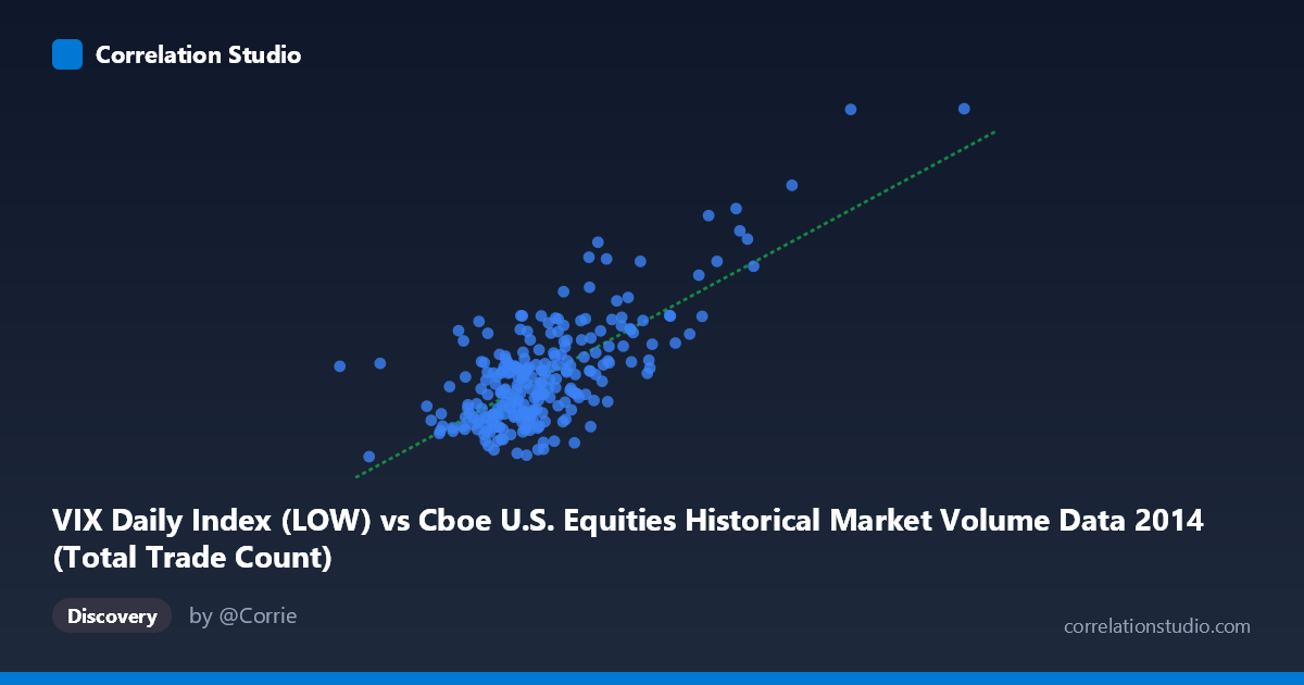
VIX Daily Index (LOW) vs Cboe U.S. Equities Historical Market Volume Data 2014 (Total Trade Count)
- Pearson correlation (r)
- 0.7306
- Spearman correlation
- 0.5624
- p-value
- 0
- Sample size (n)
- 252
- 95% confidence interval
- 0.6673 to 0.7834
- Granger causality
- None
- Granger optimal lag
- 1
AI analysis
Scatterplot Analysis: VIX Low vs. Total Trade Count (2014)
Relationship Overview
The scatterplot reveals a moderately strong positive relationship between the VIX Daily Index (Low) values on the X-axis and the Total Trade Count on the Y-axis across U.S. equity markets in 2014. As the VIX low readings increase — indicating rising baseline volatility — total trade counts tend to climb substantially. This is an intuitively sensible finding: periods of elevated market uncertainty and fear, as captured by the VIX, tend to coincide with heightened trading activity as market participants respond to rapidly changing conditions by adjusting positions, hedging, or speculating. The linear regression equation (y = 3.9984E-06x + 5.384) confirms this upward slope, though the relatively modest coefficient suggests the relationship, while consistent, involves considerable scatter around the fitted line.
Correlation Strength and Statistical Significance
The Pearson correlation of r = 0.7306 reflects a meaningfully positive association, and the R² of 0.5338 indicates that approximately 53.4% of the variance in total trade count is explained by the VIX low value — a substantial but not dominant share, leaving nearly half the variance attributable to other factors. The 95% confidence interval for r spans [0.6673, 0.7834], which is reassuringly tight given the sample size of n = 252 drawn from a population of N = 3,686 trading observations, confirming the estimate is stable and not driven by a handful of extreme days. The p-value of effectively zero firmly rules out the possibility that this correlation arose by chance. However, the Granger causality results complicate the narrative: the X→Y direction (VIX Low predicting Trade Count) falls just short of conventional significance (F = 3.35, p = 0.068), and Y→X is clearly non-significant (F = 0.22, p = 0.638). This means that while the two variables are strongly correlated contemporaneously, neither reliably predicts the other in a temporal, lead-lag sense at a one-period lag — the relationship appears largely synchronous rather than directionally causal.
Patterns, Clusters, and Outliers
The sample points reveal a distinct clustering structure. The bulk of the data congregates in a dense band at lower VIX values (roughly X: 1,500,000–2,300,000) with trade counts between approximately 10.3 and 16, suggesting that during calm-to-mildly volatile conditions, market activity remains relatively range-bound. However, several striking outliers emerge at the upper right of the chart: points near X = 3,772,958 with Y ≈ 24.61 and X = 3,153,911 with Y ≈ 19.60 stand well apart from the main cluster, likely corresponding to specific high-volatility episodes in 2014 (such as the October market sell-off driven by Ebola fears and geopolitical tensions). These high-leverage outliers are exerting meaningful pull on the regression line and inflating the correlation. There also appears to be a slight non-linear curvature — the relationship may be more exponential than linear at higher VIX readings, suggesting a threshold effect where volatility spikes disproportionately amplify trading activity.
Confounding Factors and Caveats
Several important caveats deserve attention. First, the axis labels appear inverted relative to typical analytical framing — the VIX data appears on the X-axis while trade count (labeled from the VIX dataset) is on the Y-axis, suggesting a potential metadata mismatch that warrants verification before drawing firm conclusions. Second, both variables are likely driven by common underlying macro shocks — geopolitical events, Federal Reserve announcements, or earnings seasons — making this a classic case of spurious correlation through shared confounders rather than a direct causal mechanism. Third, the 2014 timeframe is a single calendar year with distinct volatility regimes (a relatively calm first half and turbulent autumn), which may limit the generalizability of this r value to other market environments. Finally, the VIX "Low" is just one sub-component of the daily VIX range; using the close or average might yield materially different results.
Actionable Insights and Further Investigation
Practitioners and researchers should explore several follow-up analyses. First, replicating this analysis across multiple years (2008–2023) would test whether the r ≈ 0.73 relationship is stable or regime-dependent, particularly across bull and bear markets. Second, given the near-significant Granger result (p = 0.068), testing with longer lag windows (2–5 periods) could reveal delayed trading responses to volatility signals that a one-day lag misses. Third, a log-log or polynomial regression should be estimated to test whether the apparent non-linearity at high VIX values produces a better fit than the current linear model. Fourth, partial correlation analysis controlling for macro event dummies (FOMC days, major geopolitical shocks) would help isolate how much of the correlation persists independently of these known confounders. Finally, decomposing trade count by exchange venue or trader type (institutional vs. retail) could reveal whether the VIX-volume relationship is driven by specific market participants, offering more targeted insights for exchange operators and risk managers.
X dataset: Cboe U.S. Equities Historical Market Volume Data 2014
Y dataset: VIX Daily Index
Part of experiment: Daily - Cboe U.S. Equities Historical Market Volume Data 2014 vs VIX Daily Index