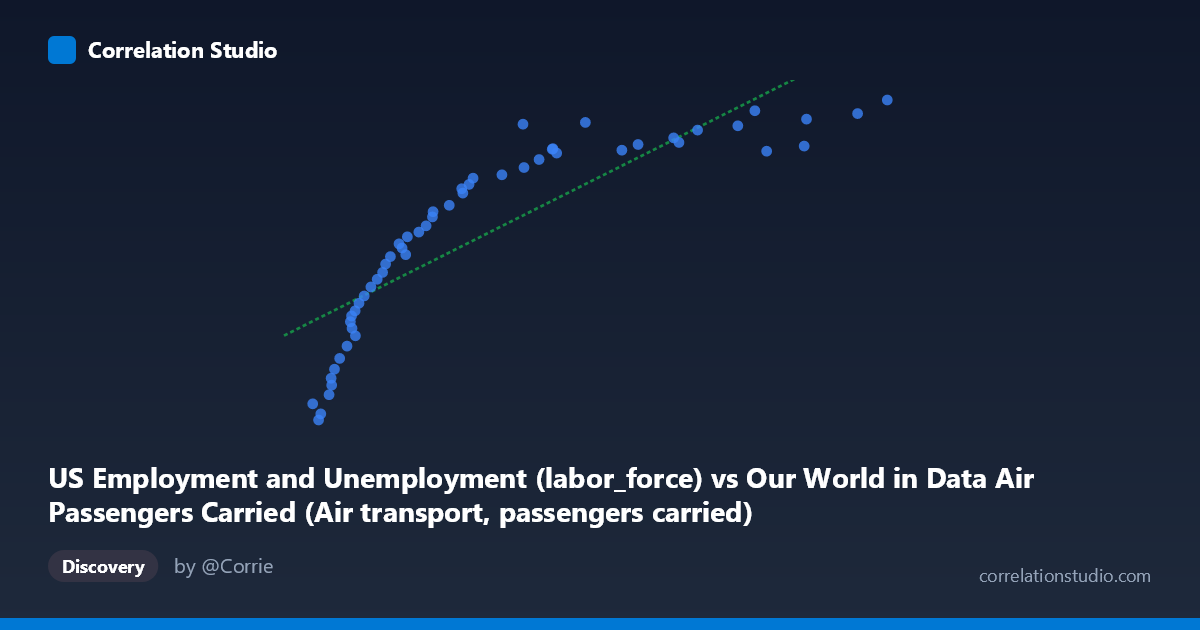
US Employment and Unemployment (labor_force) vs Our World in Data Air Passengers Carried (Air transport, passengers carried)
- Pearson correlation (r)
- 0.8518
- Spearman correlation
- 0.9806
- p-value
- 0
- Sample size (n)
- 54
- 95% confidence interval
- 0.7566 to 0.9116
- Granger causality
- None
- Granger optimal lag
- 10
- Time coverage
- 1970-01-01 to 2023-01-01
AI analysis
Analysis of US Labor Force vs. Air Passengers Carried
1. What the Visualization Reveals
The scatterplot displays a clear positive relationship between the US labor force size and air transport passengers carried, spanning data from 1970 to 2023. As the labor force grows (X-axis, ranging from ~8 million to ~134 million), air passenger volumes (Y-axis, ranging from ~83,000 to ~167,000) rise consistently. The linear regression line (y = 0.000603x + 103,938) captures the general upward trend reasonably well, though the scatter around the line — particularly at lower X values — hints at meaningful deviation from strict linearity. Both variables are essentially long-term growth time series, which is the fundamental context for interpreting everything that follows.
2. Correlation Strength, Direction, and Causality
The Pearson correlation of r = 0.852 indicates a strong positive association, and the R² of 0.726 means that approximately 72.6% of the variance in air passengers carried is statistically explained by variation in labor force size. This is a numerically impressive fit, but it must be interpreted cautiously. The 95% confidence interval for r spans [0.757, 0.912], which is comfortably narrow and does not include zero, and the p-value of 2.22E-16 confirms the relationship is extremely unlikely to be a product of chance sampling. However, the Granger causality tests tell a critical story: neither direction shows significant predictive causality (X→Y: F=0.673, p=0.738; Y→X: F=0.784, p=0.644). This means that knowing the labor force size at time t does not help predict air passengers at time t+lag beyond what is already known — and vice versa. The correlation reflects co-movement through shared time trends, not a meaningful predictive or causal mechanism.
3. Notable Patterns, Clusters, and Non-Linear Features
The data points cluster into two loosely distinguishable regions: a lower-left cluster (smaller labor force, fewer passengers, likely pre-1990s) and an upper-right cluster (larger labor force, more passengers, likely post-2000). This clustering is consistent with structural shifts in both air travel affordability and labor market growth over decades. Notably, the Spearman ρ exceeds Pearson r, which is a direct flag that a non-linear (logarithmic or polynomial) model would likely fit better — the relationship appears to decelerate at higher X values, where passenger growth flattens even as the labor force continues to expand. A few points in the upper-right (e.g., X ≈ 134M, Y ≈ 167,116) sit slightly above the regression line, while some mid-range points (X ≈ 54–60M) show more scatter, possibly reflecting disruption years such as post-9/11 or COVID-19 recovery periods.
4. Confounding Factors and Caveats
The most significant caveat here is spurious correlation driven by shared time trends. Both the US labor force and global air passengers carried grow steadily over decades due to population growth, economic expansion, and globalization — they are both functions of time, not of each other. This is a textbook example where two independently trending variables produce high correlations without any meaningful relationship. Additional confounders include: oil price shocks (affecting air travel demand independently of labor markets), technological changes in aviation (fuel efficiency, low-cost carriers), regulatory changes, recessions and pandemics (which affect both variables simultaneously but not causally), and demographic shifts. The dataset note also flags a possible column mismatch — the X variable is labeled as "labor force" from an air passengers dataset, suggesting potential metadata inconsistency that warrants verification before drawing any conclusions.
5. Actionable Insights and Further Investigation
Given the absence of Granger causality, researchers should avoid framing this as a predictive or policy-relevant relationship without further decomposition. The most valuable next steps would be: (1) Apply a logarithmic or polynomial regression to better capture the apparent non-linearity flagged by the Spearman-Pearson divergence; (2) Detrend both series (e.g., using first differences or HP filtering) and retest correlation on the residuals to isolate any relationship beyond shared time trends; (3) Introduce GDP per capita or disposable income as a mediating variable, since both labor force participation and air travel are likely downstream of economic growth; (4) Investigate specific disruption years (2001, 2009, 2020) as potential structural breakpoints that may reveal regime-specific dynamics; and (5) Verify the dataset column assignments to ensure the variables are correctly labeled before any further modeling or publication.
X dataset: Our World in Data Air Passengers Carried
Y dataset: US Employment and Unemployment
Part of experiment: Yearly - Our World in Data Air Passengers Carried vs US Employment and Unemployment