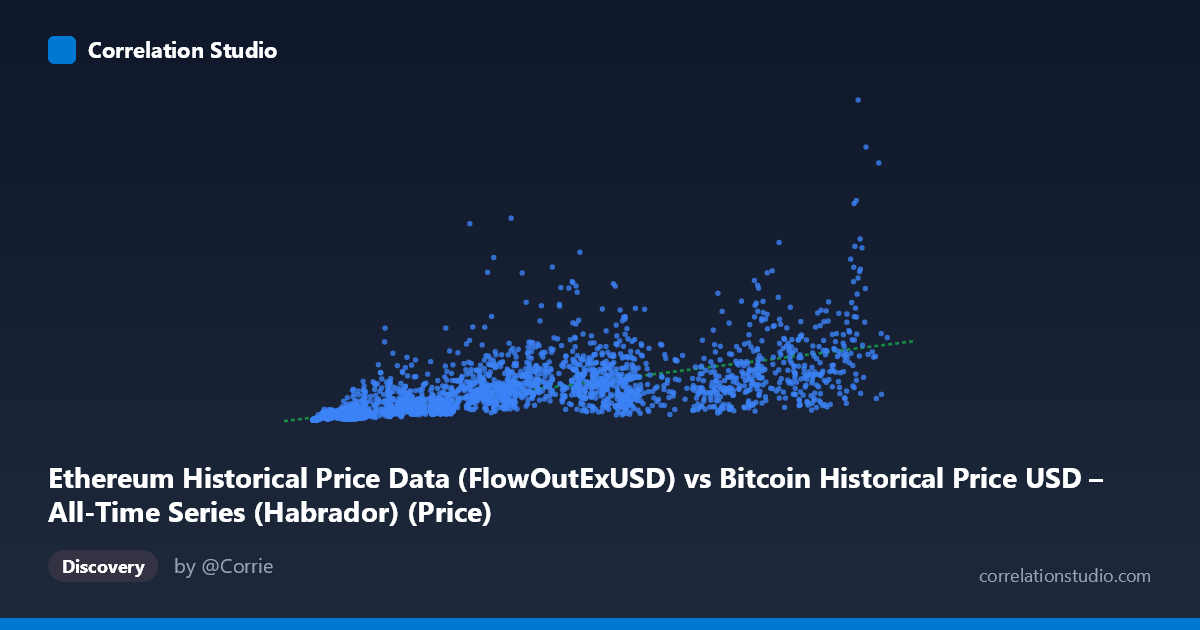
Ethereum Historical Price Data (FlowOutExUSD) vs Bitcoin Historical Price USD – All-Time Series (Habrador) (Price)
- Pearson correlation (r)
- 0.7133
- Spearman correlation
- 0.8996
- p-value
- 0
- Sample size (n)
- 3917
- 95% confidence interval
- 0.6975 to 0.7283
- Granger causality
- None
- Granger optimal lag
- 10
- Time coverage
- 2015-08-08 to 2026-04-28
AI analysis
Analysis: Ethereum Flow-Out vs. Bitcoin Price Relationship
1. Overview of the Relationship
The scatterplot depicts a positive association between an Ethereum exchange flow-out metric (X) and Bitcoin's USD price (Y) across 3,917 paired daily observations spanning 2015–2026. Both variables exhibit extreme right-skew — X ranges from ~209 to ~124,720 with a mean of 30,520 but stdev of 32,543 (nearly equal to the mean), while Y ranges from ~$14K to ~$7.36B with a mean of $465M and stdev of $615M (stdev exceeding the mean). This signals heavy-tailed distributions with a small number of very large values dominating the scale, which is typical of cryptocurrency price/volume data pooled across bull and bear cycles.
2. Correlation Strength and Statistical Confidence
The Pearson correlation (r = 0.713) indicates a moderately strong positive linear relationship, with r² = 0.509 meaning roughly 51% of the variance in Bitcoin price is statistically associated with variance in the Ethereum flow-out metric — leaving nearly half unexplained. The 95% CI [0.698, 0.728] is tight, and p ≈ 0 confirms this correlation is highly unlikely to be due to chance at this sample size. However, statistical significance here reflects the large N more than practical strength — r² of ~0.51 is a moderate, not tight, fit.
Critically, the Granger causality tests show no significant predictive direction in either direction (X→Y: p=0.14; Y→X: p=0.23). This is an important caveat: despite the strong contemporaneous correlation, neither series reliably leads the other in time. This strongly suggests the correlation is driven by a shared underlying trend or common macro factor (e.g., both assets rising/falling together during crypto market cycles) rather than one variable causally forecasting the other.
3. Patterns, Clustering, and Non-linearity
The data shows a fan-shaped/heteroskedastic pattern — variance in Y increases substantially as X increases, visible in the sample points (e.g., at X≈42,000–45,000, Y ranges from $556M to $1.76B). Several notable outliers exist: (118,410, $7.36B) is far above the general trend, while points like (70,707, $229M) or (93,784, $280M) fall well below it despite high X values. The note that Spearman ρ exceeds Pearson r is a key signal — it indicates the relationship is monotonic but not well-captured by a straight line; a log-log or power-law transformation is likely more appropriate given the multiplicative, skewed nature of both variables (common in financial/crypto data where percentage changes matter more than absolute ones).
4. Confounding Factors and Caveats
The most significant confound is that both variables are crypto-asset metrics likely driven by the same macro market cycles (bull/bear regimes, overall risk sentiment, BTC dominance shifts) rather than one causing the other. Time-series autocorrelation is another concern: consecutive daily observations are not independent, which can artificially inflate correlation and violate the i.i.d. assumptions underlying the p-value/CI calculations. Additionally, using raw (non-detrended) price levels across an 11-year span mixes multiple distinct market regimes (2015 lows vs. 2021/2024 highs), which can create spurious correlation purely from shared long-term upward drift rather than genuine linkage.
5. Recommendations for Further Investigation
1. Log-transform both axes and refit — given the skew and Spearman/Pearson discrepancy, a log-log regression will likely show a better-fitting, more interpretable power-law relationship. 2. Detrend or difference the series (e.g., use daily returns/% changes instead of levels) to remove shared drift and test whether the correlation persists — this better isolates genuine co-movement from mutual trend. 3. Segment by market regime (bull vs. bear cycles) to check if the relationship is stable or regime-dependent. 4. Investigate the outlier at (118,410, $7.36B) and other high-leverage points, as they may disproportionately influence the linear fit. 5. Given the null Granger result, avoid using this X variable as a predictive/forecasting input for BTC price; instead, treat the relationship as descriptive/contemporaneous co-movement.
X dataset: Bitcoin Historical Price USD – All-Time Series (Habrador)
Y dataset: Ethereum Historical Price Data
Part of experiment: Bitcoin - Bitcoin Historical Price USD – All-Time Series (Habrador) vs Ethereum Historical Price Data