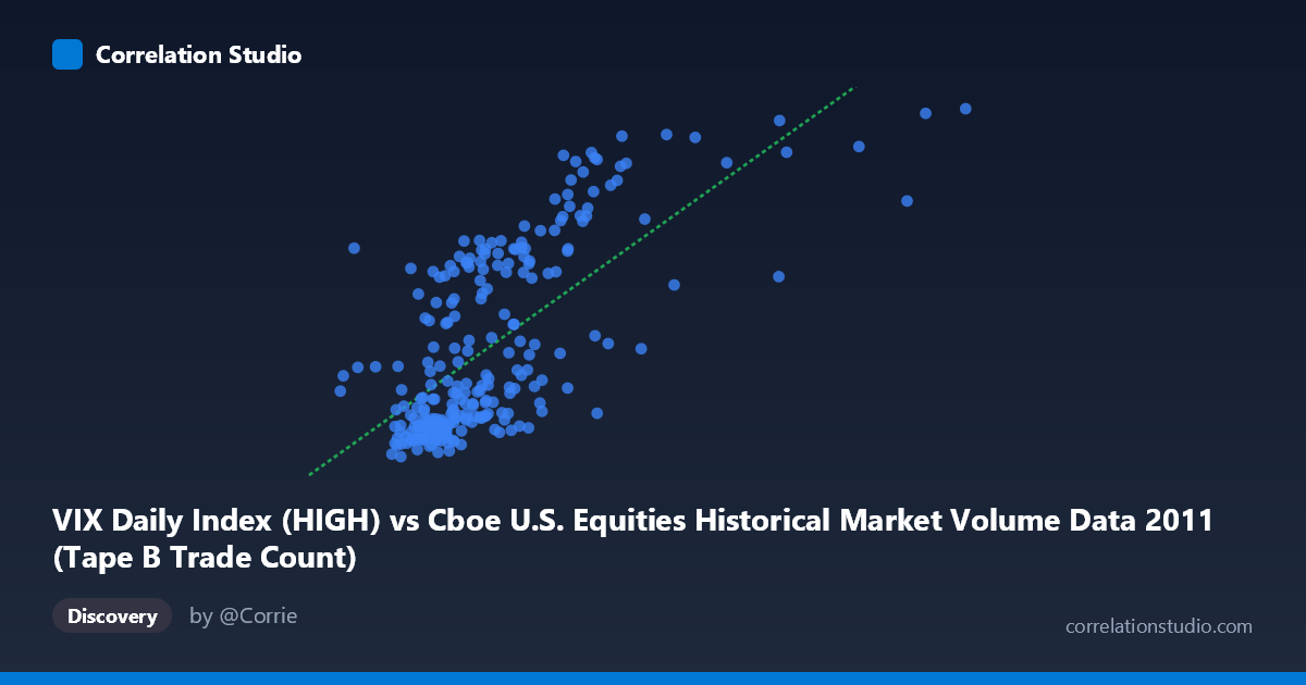
VIX Daily Index (HIGH) vs Cboe U.S. Equities Historical Market Volume Data 2011 (Tape B Trade Count)
- Pearson correlation (r)
- 0.6965
- Spearman correlation
- 0.685
- p-value
- 0
- Sample size (n)
- 252
- 95% confidence interval
- 0.6269 to 0.7551
- Granger causality
- None
- Granger optimal lag
- 1
AI analysis
Scatterplot Analysis: VIX High vs. Tape B Trade Count (2011)
Relationship Overview The scatterplot reveals a moderately strong positive relationship between the CBOE VIX Daily Index (High) and Tape B Trade Count across U.S. equities exchanges in 2011. As the VIX high values increase — indicating rising market fear or uncertainty — Tape B trade counts tend to rise correspondingly. This pattern is economically intuitive: periods of elevated volatility typically drive heightened trading activity as market participants rebalance portfolios, hedge positions, or react to news events. The linear regression equation (y = 5.84e-05x + 8.96) suggests a modest but consistent slope, meaning each unit increase in VIX high is associated with a measurable uptick in trade volume activity on Tape B venues.
Correlation Strength and Statistical Significance The Pearson correlation of r = 0.6965 indicates a moderately strong positive association, but the r² of 0.4851 is the more telling statistic — approximately 48.5% of the variance in Tape B trade counts is explained by VIX high values, meaning nearly half the variation remains unexplained by this relationship alone. The 95% confidence interval of [0.6269, 0.7551] is relatively tight given the sample size of n = 252, and the p-value of effectively zero confirms this correlation is highly unlikely to be a chance finding within this dataset. However, the Granger causality results are notably unremarkable: neither direction (X→Y: F = 0.2505, p = 0.617; Y→X: F = 0.2523, p = 0.616) approaches significance at any conventional threshold. This means that while the two variables co-move, neither reliably predicts the other one lag period ahead — the relationship appears contemporaneous and possibly driven by shared external forces rather than one series causally leading the other.
Notable Patterns, Clusters, and Outliers The sample points reveal a recognizable clustering structure. A dense cluster of observations sits in the lower-left region — VIX values roughly between 109,000–250,000 paired with trade counts in the 16–22 range — suggesting that calm, low-volatility periods dominated much of 2011. A second, more diffuse cluster occupies the upper-right quadrant (VIX highs above 350,000, trade counts above 30), consistent with the well-documented volatility spikes of mid-to-late 2011 tied to the U.S. debt ceiling crisis and European sovereign debt concerns. Several apparent outliers are visible, including observations near (556,197, 42.88) and (495,413, 31.28), which may correspond to specific stress events. Notably, the spread of trade counts increases at higher VIX levels, hinting at heteroscedasticity — the relationship becomes noisier as volatility rises, which is a meaningful caveat for the linear model's applicability across the full range.
Confounding Factors and Caveats Several important caveats temper interpretation. First, 2011 was an unusually volatile year with discrete macro shocks (debt ceiling, eurozone crisis, S&P downgrade of U.S. debt), which may have created a spurious or regime-specific correlation that does not generalize to other years. Second, Tape B specifically covers NYSE American (AMEX) and regional exchange-listed securities — a subset of total market volume — so the relationship may not extrapolate to Tape A or C. Third, the absence of Granger causality suggests both variables may be jointly driven by a latent factor (e.g., macro news flow, institutional risk-on/risk-off behavior), making causal inference from this correlation alone inappropriate. Fourth, the use of VIX high (rather than close or average) may amplify intraday spikes, potentially inflating the apparent co-movement on extreme days.
Actionable Insights and Further Investigation Practitioners could explore whether this relationship holds across multiple years to test its robustness beyond 2011's unique macro environment. Introducing a regime-switching model or segmenting the data by volatility quartile would help quantify whether the relationship strengthens nonlinearly above a VIX threshold — the visible heteroscedasticity suggests this is likely. Including additional predictors (e.g., S&P 500 returns, bid-ask spreads, news sentiment scores) could push r² substantially above the current 48.5% ceiling and better isolate the VIX effect. Finally, examining Granger causality at longer lags (e.g., 5 or 10 periods) or using intraday data might reveal predictive dynamics that the daily lag-1 test missed, and could help distinguish whether elevated VIX anticipates volume surges or merely accompanies them.
X dataset: Cboe U.S. Equities Historical Market Volume Data 2011
Y dataset: VIX Daily Index
Part of experiment: Daily - Cboe U.S. Equities Historical Market Volume Data 2011 vs VIX Daily Index