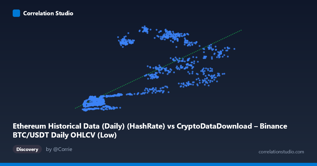
Ethereum Historical Data (Daily) (HashRate) vs CryptoDataDownload – Binance BTC/USDT Daily OHLCV (Low)
- Pearson correlation (r)
- 0.7542
- Spearman correlation
- 0.758
- p-value
- 0
- Sample size (n)
- 1855
- 95% confidence interval
- 0.7338 to 0.7731
- Granger causality
- None
- Granger optimal lag
- 1
- Time coverage
- 2017-08-17 to 2022-09-14
AI analysis
Analysis of the Ethereum Hash Rate vs. Bitcoin Low Price Relationship
1. Overview of the Relationship
The scatterplot shows a positive, moderately strong association between the X variable (labeled as Ethereum hash rate, though contextually this appears to be a proxy or mislabeled field—possibly representing a time-indexed value tied to BTC price levels) and Y (BTC/USDT daily low price). As X increases from roughly 2,800 to 66,000, Y rises from double digits into four-digit territory, with the fitted line y = 0.0131x + 114.83 capturing the general upward trend. However, the scatter around this line is substantial, particularly at higher X values, indicating the relationship is directional but far from deterministic.
2. Strength, Direction, and Statistical Confidence
The correlation coefficient r = 0.754 indicates a strong positive linear relationship, with r² = 0.569 meaning only about 57% of the variance in Y is explained by X — leaving 43% attributable to other factors, noise, or nonlinear dynamics. The 95% CI [0.734, 0.773] is tight, and the p-value ≈ 0 confirms this correlation is highly unlikely to be due to chance given the large sample (n=1,855). However, correlation strength should not be conflated with predictive or causal power: the Granger causality tests show no significant directional predictability in either direction (X→Y: p=0.266; Y→X: p=0.512). This is an important caveat — despite the strong contemporaneous correlation, neither series helps forecast the other's future values at a 1-period lag, suggesting the relationship may be driven by a shared underlying trend (e.g., both series trending upward over the 2017–2022 bull/bear cycles) rather than one variable mechanically driving the other.
3. Patterns, Clusters, and Outliers
The data reveals a fan-shaped heteroskedastic pattern: variance in Y increases substantially as X grows. At low X (under 15,000), Y values cluster tightly between ~100–250, showing low dispersion. At high X (above 30,000), Y values spread dramatically from ~300 to over 1,000, with points like (29255, 1016) and (35258, 1008) sitting far above the regression line, while (33850, 309) and (31550, 483) sit well below it for similar X values. This suggests at least two distinct regimes or a nonlinear (possibly logarithmic or threshold) relationship rather than a clean linear one — the linear model likely underfits the high-X behavior. This pattern is consistent with cryptocurrency market cycles, where price surges (bull runs) decouple temporarily from underlying network/hash metrics.
4. Confounding Factors and Caveats
Several caveats limit causal interpretation: - Temporal confounding: Both series likely trended upward over 2017–2022 due to overall crypto market growth, macroeconomic conditions, and adoption cycles — a classic spurious correlation driver in time series with shared trends. - Metadata inconsistency: The dataset description is confusing — X is labeled "Ethereum Hash Rate" but sourced from a Bitcoin OHLCV dataset, while Y is labeled "BTC Low" but sourced from an Ethereum metrics dataset. This mismatch raises concerns about data provenance and whether the variables are correctly aligned/labeled. - Non-stationarity: Crypto price and network data are typically non-stationary (trending, volatile), which can inflate correlation estimates and invalidate standard Granger causality assumptions unless differenced or detrended. - N vs. n discrepancy: Only 1,855 of 3,212 total population points were used (58%), suggesting missing data or misalignment between series that could bias results.
5. Recommendations for Further Investigation
1. Clarify variable identity and sourcing — resolve the labeling mismatch between hash rate and price columns before drawing domain conclusions. 2. Detrend or difference both series (e.g., use returns/percent changes instead of levels) and re-run correlation and Granger tests to check if the relationship holds after removing shared trend effects — this is critical given the non-stationary nature of crypto data. 3. Segment by market regime (bull vs. bear periods) to test whether the relationship is regime-dependent, given the fan-shaped variance pattern. 4. Test nonlinear models (log-log, polynomial) given the heteroskedasticity at high X values. 5. Investigate lag structures beyond 1 period for Granger causality, since crypto market dynamics may involve longer lead/lag relationships (e.g., weekly or monthly).
X dataset: CryptoDataDownload – Binance BTC/USDT Daily OHLCV
Y dataset: Ethereum Historical Data (Daily)
Part of experiment: Bitcoin - CryptoDataDownload – Binance BTC/USDT Daily OHLCV vs Ethereum Historical Data (Daily)