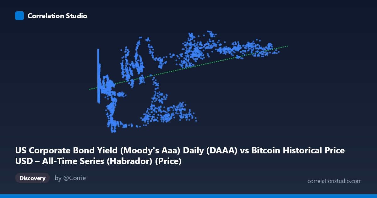
US Corporate Bond Yield (Moody's Aaa) Daily (DAAA) vs Bitcoin Historical Price USD – All-Time Series (Habrador) (Price)
- Pearson correlation (r)
- 0.4494
- Spearman correlation
- 0.2041
- p-value
- 0
- Sample size (n)
- 4042
- 95% confidence interval
- 0.4245 to 0.4737
- Granger causality
- X → Y
- Granger optimal lag
- 1
- Time coverage
- 2010-07-19 to 2026-09-15
- Recomputed on refreshed data
- 2026-10-24 (r was 0.4494)
AI analysis
Analysis: Bitcoin Price vs. Moody's Aaa Corporate Bond Yield
1. What the Visualization Reveals
Despite the axis labels being somewhat crossed in the metadata (X is labeled as the bond yield dataset but the values 0.05–124,720 clearly represent Bitcoin price, while Y ranges 2.01–5.80 which matches bond yield percentages), the data shows Bitcoin price plotted against Aaa corporate bond yields over a ~16-year span (2010–2026). The scatter shows a loose, positive-sloping cloud rather than a tight linear band. At low Bitcoin prices (under a few hundred dollars), yields vary widely (3.5–5.3%), reflecting the early Bitcoin era spanning multiple bond-market regimes. At high Bitcoin prices ($60,000), yields cluster more tightly in the 4.9–5.7% range, suggesting these observations are concentrated in a specific recent period of elevated corporate yields.
2. Strength, Direction, and Uncertainty
The correlation coefficient (r = 0.41) indicates a moderate positive relationship, but r² = 0.167 means only about 16.7% of the variance in bond yields is explained by Bitcoin price (or vice versa) — leaving over 83% unexplained by this bivariate relationship alone. The 95% CI [0.382, 0.434] is fairly narrow given the large sample (n=3,946), and the p-value ≈ 0 confirms the correlation is statistically distinguishable from zero — but statistical significance here reflects sample size more than practical strength. Critically, the Granger causality tests show no significant predictive direction: X→Y is marginal (p=0.082) and Y→X is clearly insignificant (p=0.339). This means neither series reliably leads the other in a temporal forecasting sense at lag 1 — the correlation is likely contemporaneous/structural rather than causal.
3. Patterns, Clusters, and Outliers
The data shows a clear temporal clustering structure rather than a smooth continuous relationship: low-price/early-era Bitcoin points (2010–2013) are scattered across the full yield range, while high-price points ($60k, likely 2021 and 2023–2026) coincide with the higher-yield regime (~5%+). This looks less like a genuine causal link and more like two independent long-term trends (Bitcoin's secular price appreciation and the bond market's post-2021 rate-hiking cycle) that happen to overlap in time. Notable outliers include high-yield/low-price points (e.g., $220 at 3.52%) and high-price/moderate-yield points (e.g., $34,574 at 2.56%), which break any clean monotonic pattern and suggest regime-dependent behavior rather than a stable functional relationship.
4. Confounding Factors and Caveats
This is a classic case of spurious correlation via shared time trend. Both Bitcoin price (largely driven by adoption, halving cycles, speculative demand) and Aaa bond yields (driven by Fed policy, inflation expectations, macro conditions) have exhibited long-term drift over the 2010–2026 window, and any two trending time series will show correlation without genuine causal linkage. The extreme right-skew of Bitcoin price (mean $20,753 vs. stdev $30,308, with a max of $124,720) means the regression is heavily influenced by a cluster of recent high-price observations. Additionally, non-stationarity in both series violates assumptions needed for meaningful correlation/Granger interpretation — these tests should ideally be run on detrended, differenced, or log-transformed data (especially given Bitcoin's exponential price behavior) rather than raw levels.
5. Suggestions for Further Investigation
Given the weak explanatory power and lack of Granger causality, this pairing should not be used for predictive trading or forecasting purposes as-is. Recommended next steps: (1) log-transform Bitcoin price given its extreme skew and multi-order-of-magnitude range; (2) test correlations on first differences or returns rather than levels to remove spurious trend-driven correlation; (3) run Granger causality on stationary (differenced) series, since level-based tests are unreliable when both series are trending; and (4) consider a third common driver (e.g., real interest rates, inflation expectations, or macro liquidity cycles) that may jointly influence both series rather than treating this as a direct bivariate relationship.
X dataset: Bitcoin Historical Price USD – All-Time Series (Habrador)
Y dataset: US Corporate Bond Yield (Moody's Aaa) Daily
Part of experiment: Bitcoin - Bitcoin Historical Price USD – All-Time Series (Habrador) vs US Corporate Bond Yield (Moody's Aaa) Daily