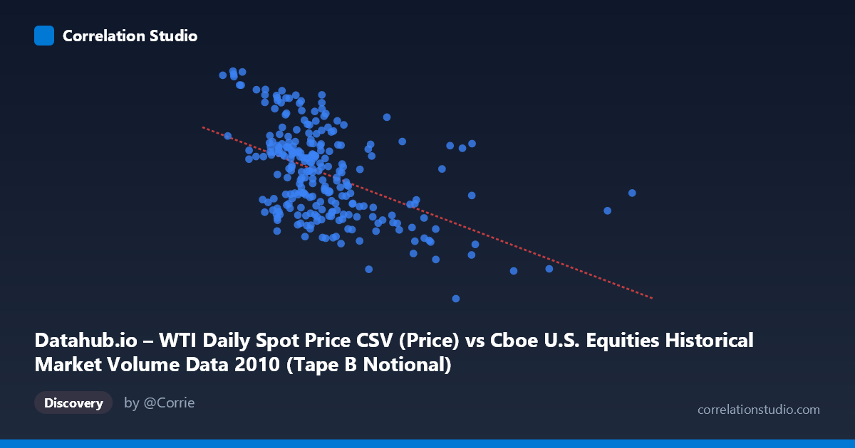
Datahub.io – WTI Daily Spot Price CSV (Price) vs Cboe U.S. Equities Historical Market Volume Data 2010 (Tape B Notional)
- Pearson correlation (r)
- -0.4909
- Spearman correlation
- -0.475
- p-value
- 0
- Sample size (n)
- 252
- 95% confidence interval
- -0.5793 to -0.391
- Granger causality
- None
- Granger optimal lag
- 1
AI analysis
Scatterplot Analysis: WTI Crude Oil Price vs. Cboe Tape B Notional Volume (2010)
Relationship Overview
The scatterplot reveals a moderate negative relationship between Cboe U.S. Equities market volume (Tape B Notional, on the X-axis) and WTI daily crude oil spot prices (on the Y-axis) across 2010 trading days. The linear regression equation (y = -1.27248E-09x + 86.04) confirms this inverse association: as equity market notional volume increases, oil prices tend to decline. This is a somewhat counterintuitive pairing at first glance, but it reflects a plausible macroeconomic dynamic — periods of elevated equity trading volume may correspond to market stress or risk-off sentiment, which can suppress commodity demand expectations and thus oil prices. The scatter of points is notably wide, however, suggesting that this relationship, while real, is far from deterministic.
Correlation Strength, Direction, and Statistical Significance
The Pearson correlation of r = -0.4909 indicates a moderate negative association, and the R² of 0.2410 means that roughly 24.1% of the variance in WTI oil prices is explained by Tape B notional volume — a meaningful but decidedly partial explanation, with approximately 76% of oil price variation attributable to other factors. The 95% confidence interval of [-0.5793, -0.3910] is entirely negative and reasonably narrow given the sample size (n = 252 paired observations from a population of N = 3,302), lending credible statistical confidence to the direction of the effect. The p-value of effectively zero confirms this is not a chance finding at conventional significance thresholds. That said, the Granger causality results complicate the narrative significantly: neither direction achieves significance at the 5% level (X→Y: F = 1.23, p = 0.269; Y→X: F = 3.29, p = 0.071). This means we cannot statistically claim that either variable temporally predicts the other with a one-period lag — the correlation exists cross-sectionally, but there is no robust evidence of a leading/lagging predictive relationship in the time series sense.
Notable Patterns, Clusters, and Outliers
Several structural features stand out in the data. There is a visible cluster of points at lower X-values (roughly 2–5 × 10⁹) that spans a wide vertical range of oil prices (~75–91 USD/barrel), suggesting that at lower trading volumes, oil prices were quite variable — likely reflecting earlier 2010 conditions before volume patterns consolidated. At higher X-values (above ~8–10 × 10⁹), oil prices compress toward the lower range (~65–76 USD/barrel), consistent with the negative regression slope. A handful of notable outliers are visible: the point near (15.1 × 10⁹, 75.10) represents an extreme volume day with a moderate oil price, and the cluster around (9.8 × 10⁹, 64.78) marks the lowest oil price in the dataset coinciding with high volume — both consistent with the negative trend but pulling leverage on the regression line. The upper-left region contains several high-oil-price, low-volume days (e.g., ~90.84 at ~2.0 × 10⁹), which likely reflect earlier 2010 periods or specific supply-demand events.
Confounding Factors and Interpretive Caveats
Several important caveats apply. First, both variables are time-indexed to 2010, meaning shared temporal trends (e.g., recovery from the 2008–2009 financial crisis, macroeconomic seasonality, or the April 2010 Deepwater Horizon oil spill) could be driving both series independently, creating a spurious or partially spurious correlation. The lack of Granger causality is a meaningful red flag here — it suggests the correlation may reflect common exposure to a third driver (e.g., macroeconomic risk sentiment, GDP expectations, or the VIX) rather than any direct mechanical link between equity trading volume and oil prices. Second, Tape B specifically covers NYSE American and regional exchange listings, which may not be the most representative proxy for broad market activity. Third, the notional volume figures span an enormous range (1.6 × 10⁹ to 16.0 × 10⁹), and the relationship may not be linear across this full range — a log transformation of X could be warranted.
Actionable Insights and Further Investigation
Given that 24% of oil price variance is associated with equity volume but temporal predictability is absent, the most productive next steps would include: (1) introducing explicit risk-sentiment proxies such as the VIX or credit spreads as control variables to test whether the correlation survives conditional on market stress; (2) applying a log or power transformation to the notional volume variable to test for a better-fitting non-linear model; (3) extending the time horizon beyond 2010 to assess whether this negative relationship is a stable structural feature or specific to the post-crisis recovery environment; and (4) testing Granger causality at longer lags (e.g., 5–10 periods) since a one-day lag may be too short to capture any real transmission mechanism between equity market activity and oil price discovery. The correlation is statistically robust but causally ambiguous, making it a useful descriptive finding that warrants deeper structural modeling before any trading or policy inference is drawn.
X dataset: Cboe U.S. Equities Historical Market Volume Data 2010
Y dataset: Datahub.io – WTI Daily Spot Price CSV
Part of experiment: Daily - Cboe U.S. Equities Historical Market Volume Data 2010 vs Datahub.io – WTI Daily Spot Price CSV