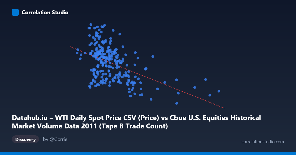
Datahub.io – WTI Daily Spot Price CSV (Price) vs Cboe U.S. Equities Historical Market Volume Data 2011 (Tape B Trade Count)
- Pearson correlation (r)
- -0.4891
- Spearman correlation
- -0.4243
- p-value
- 0
- Sample size (n)
- 252
- 95% confidence interval
- -0.5777 to -0.389
- Granger causality
- None
- Granger optimal lag
- 1
AI analysis
Analysis: WTI Oil Price vs. Cboe Tape B Trade Count (2011)
Relationship Overview The scatterplot reveals a moderate negative relationship between WTI daily spot prices (X-axis) and Cboe U.S. Equities Tape B trade counts (Y-axis) across 252 trading days in 2011. The linear regression equation (y = -3.77×10⁻⁵x + 105.496) indicates that as WTI oil prices increase, Tape B trade counts tend to decline. Visually, the data points form a downward-sloping cloud, with higher oil prices generally clustering toward lower trade counts, though considerable scatter surrounds this trend. The relationship is real but far from deterministic, suggesting meaningful noise and likely competing influences operating simultaneously throughout the year.
Correlation Strength and Statistical Significance The Pearson correlation of r = -0.489 reflects a moderate negative association. More precisely, R² = 0.239 means that WTI oil prices explain roughly 23.9% of the variance in Tape B trade counts — a non-trivial but decidedly incomplete explanation, leaving ~76% of variance attributable to other factors. The 95% confidence interval of [-0.578, -0.389] is meaningfully bounded away from zero, and the p-value of 2.22×10⁻¹⁶ confirms the relationship is highly statistically significant given the population of N = 3,780 with n = 252 sampled pairs. However, statistical significance here should not be conflated with practical magnitude — the effect size is modest. Crucially, Granger causality analysis finds no significant predictive direction: X→Y yields F = 0.005, p = 0.945 (essentially zero predictive power), and Y→X yields F = 3.14, p = 0.078 (marginally suggestive but below conventional thresholds). This means that neither variable reliably predicts future values of the other at a one-period lag, undermining any causal narrative despite the cross-sectional correlation.
Notable Patterns, Clusters, and Outliers Several structural features are visible in the data. A distinct cluster of observations concentrates in the X range of roughly 175,000–330,000 (lower-to-mid oil price zone) with Tape B counts spanning a wide band from ~85 to ~113, suggesting high variability in trading activity even at similar price levels. At higher oil price values (above ~450,000), the scatter thins considerably and trade counts appear more uniformly suppressed, roughly in the 80–98 range. A few potential outliers warrant attention: the point near (174,908, 111.68) represents an unusually high trade count at a relatively low price, and (293,331, 110.60) sits well above the regression line at a moderate price. Conversely, (381,544, 78.93) and (390,106, 81.87) register notably low trade counts at elevated prices, reinforcing the negative trend at the upper end of the distribution.
Confounding Factors and Interpretive Caveats Several important caveats apply. First, 2011 was a distinctive macro year — marked by the Arab Spring driving oil price spikes, the European sovereign debt crisis, and the U.S. debt ceiling standoff — meaning that both variables were responding to shared macro shocks rather than necessarily influencing each other directly. This classic omitted variable problem (e.g., risk sentiment, VIX levels, global macro uncertainty) likely explains much of the observed correlation. Second, Tape B specifically covers NYSE American (AMEX) and regional exchange listings, which may respond differently to commodity price shocks than broader market indices — the correlation may not generalize to Tape A or C. Third, the dataset note fields are inverted (X and Y descriptions appear swapped in the metadata), which raises a data attribution flag requiring verification before drawing firm conclusions. Finally, the Granger causality result is a strong reminder that correlation in levels does not imply dynamic predictive relationships.
Actionable Insights and Further Investigation Despite the absence of Granger causality, the moderate R² suggests oil prices carry genuine contemporaneous information about equity trading activity in this segment, which could be useful for same-day volume modeling. Analysts should consider controlling for macro confounders — particularly VIX, S&P 500 returns, and USD/barrel volatility — to isolate whether the oil-volume relationship persists on a residual basis. Testing with longer lag structures (beyond one period) or using rolling-window Granger tests could reveal time-varying predictive relationships that a fixed one-lag analysis misses. It would also be valuable to replicate this analysis across multiple years to determine whether 2011's elevated oil price environment created an unusually strong negative relationship, or whether this is a stable structural feature. Finally, investigating whether energy sector stocks within Tape B drive the aggregate relationship — or whether it reflects broader risk-off trading behavior — would sharpen the practical interpretation considerably.
X dataset: Cboe U.S. Equities Historical Market Volume Data 2011
Y dataset: Datahub.io – WTI Daily Spot Price CSV
Part of experiment: Daily - Cboe U.S. Equities Historical Market Volume Data 2011 vs Datahub.io – WTI Daily Spot Price CSV