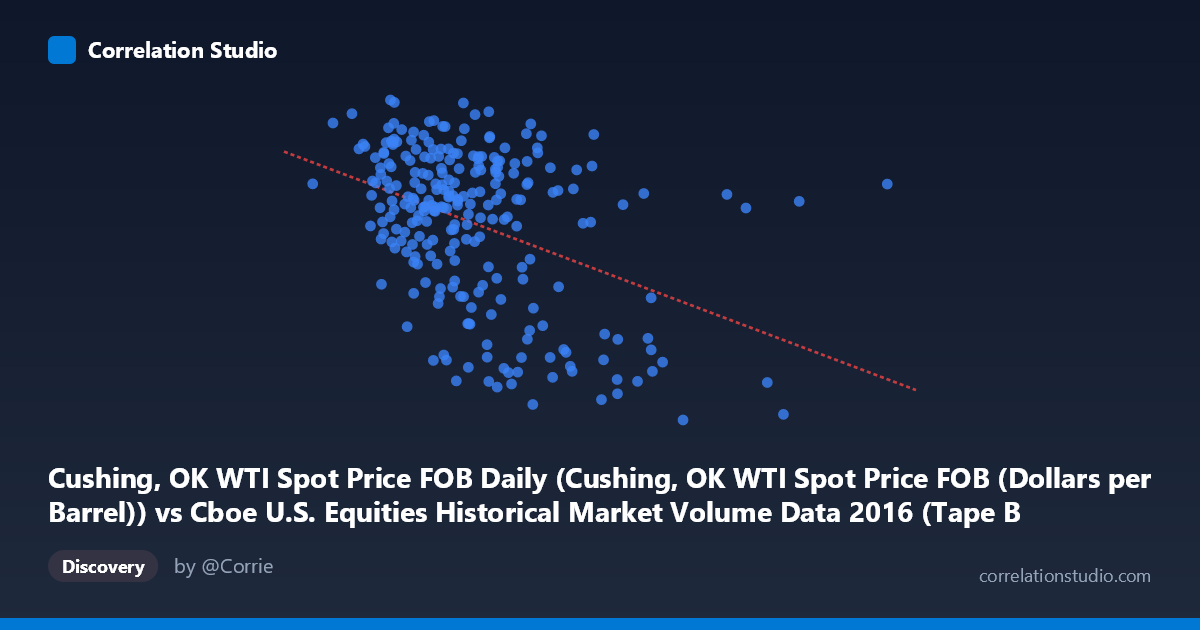
Cushing, OK WTI Spot Price FOB Daily (Cushing, OK WTI Spot Price FOB (Dollars per Barrel)) vs Cboe U.S. Equities Historical Market Volume Data 2016 (Tape B Notional)
- Pearson correlation (r)
- -0.4087
- Spearman correlation
- -0.3439
- p-value
- 0
- Sample size (n)
- 252
- 95% confidence interval
- -0.5067 to -0.3003
- Granger causality
- None
- Granger optimal lag
- 1
AI analysis
Analysis: WTI Crude Oil Spot Price vs. Cboe Tape B Notional Volume (2016)
Relationship Overview
The scatterplot reveals a modest negative relationship between Cushing, OK WTI Spot Price (X-axis) and Cboe Tape B Notional trading volume (Y-axis) across 252 trading days in 2016. The linear regression equation (y = -1.77×10⁻⁹x + 52.20) captures a downward slope, suggesting that as WTI oil prices increased, Tape B notional volume tended to decrease. Visually, the cloud of points shows a discernible but noisy downward trend, with considerable scatter around the regression line — consistent with a correlation that is real but far from deterministic.
Correlation Strength and Statistical Significance
The correlation coefficient of r = -0.41 indicates a weak-to-moderate negative association. Critically, R² = 0.167 means only 16.7% of the variance in Tape B notional volume is explained by WTI prices, leaving roughly 83% attributable to other factors. The 95% confidence interval of [-0.51, -0.30] is meaningfully below zero throughout, and the p-value of 1.45×10⁻¹¹ confirms this is highly statistically significant — very unlikely to be a chance finding given n = 252. However, despite statistical significance, the Granger causality tests show no significant temporal predictive direction in either direction (X→Y: F = 0.65, p = 0.42; Y→X: F = 0.56, p = 0.45). This is an important distinction: while the two variables co-vary, neither reliably predicts the other with a one-period lag, meaning the relationship appears contemporaneous rather than causal or leading/lagging.
Notable Patterns, Clusters, and Outliers
Several features stand out in the sample data. There is a visible cluster of points in the X range of roughly 3.5–5.5 billion (WTI prices ~$35–$55/barrel) where Tape B volume spans a wide range (approximately 38–52), creating a dense, diffuse cloud that weakens the apparent linear fit. At higher WTI price values (X 7–8 billion range), a small number of points appear as low-Y outliers — for example, coordinates near (8,085B, 29.55) and (8,201B, 45.88) — suggesting that at elevated price levels, notional volume either collapses or remains elevated in isolated instances. These high-X, low-Y outliers likely exert disproportionate influence on the regression slope and may warrant further scrutiny as leverage points.
Confounding Factors and Caveats
Several important caveats apply. First, 2016 was a highly unusual year for both oil markets and equity trading, with WTI recovering from multi-year lows (~$26/barrel in February) to ~$54 by year-end — this structural trend could create spurious correlation through shared time trends rather than a direct economic link. Second, Tape B notional volume reflects trading on specific regional exchanges, and its behavior is driven by broad equity market dynamics, index rebalancing, and algorithmic activity that may have only incidental relationships with energy prices. Third, the population size of N = 3,622 versus n = 252 sampled pairs suggests aggregation or sampling decisions that could affect representativeness. Finally, the axis labels appear to be swapped in the dataset description (X is labeled from the Cboe dataset, Y from the WTI dataset), which should be verified before drawing firm conclusions.
Actionable Insights and Further Investigation
Given the modest but statistically significant correlation, practitioners should avoid over-interpreting this as a predictive or causal signal — the Granger results explicitly rule that out at lag-1. Further investigation should include: (1) testing longer lags in Granger causality (e.g., 5- or 10-day) to capture slower-moving energy-to-equity transmission; (2) decomposing the time series to remove shared trending components and re-testing correlation on detrended or differenced data; (3) examining whether the relationship strengthens during specific regimes (e.g., periods of oil price shock vs. stability); and (4) including control variables such as VIX, overall market volume, or broader commodity indices to assess whether the oil-volume link survives multivariate scrutiny. The outlier cluster at high X values deserves targeted investigation to determine whether they represent data anomalies or genuine market events.
X dataset: Cboe U.S. Equities Historical Market Volume Data 2016
Y dataset: Cushing, OK WTI Spot Price FOB Daily
Part of experiment: Daily - Cboe U.S. Equities Historical Market Volume Data 2016 vs Cushing, OK WTI Spot Price FOB Daily