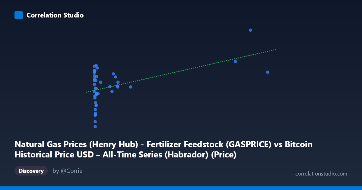
Natural Gas Prices (Henry Hub) - Fertilizer Feedstock (GASPRICE) vs Bitcoin Historical Price USD – All-Time Series (Habrador) (Price)
- Pearson correlation (r)
- 0.4961
- Spearman correlation
- 0.1122
- p-value
- 0.000716
- Sample size (n)
- 43
- 95% confidence interval
- 0.23 to 0.6932
- Granger causality
- None
- Granger optimal lag
- 1
AI analysis
Analysis: Natural Gas Prices vs. Bitcoin Historical Price
1. What the Visualization Reveals
The scatterplot shows a heavily right-skewed distribution along the X-axis (natural gas feedstock prices), with the vast majority of observations clustered below X=200, and a handful of extreme outliers extending out to nearly 950. The Y-axis (labeled as Bitcoin price, though values range 1.95–6.01, suggesting this is likely a transformed/normalized or mislabeled series rather than raw USD price) shows a much tighter, more normally-distributed spread. The overall pattern suggests a modest positive association: as X increases, Y tends to drift upward, but with substantial scatter at every X value, especially in the dense low-X cluster.
2. Strength, Direction, and Statistical Confidence
The correlation coefficient (r = 0.496) indicates a moderate positive relationship, but r² = 0.246 tells the more important story: only about 24.6% of the variance in Y is explained by X, leaving roughly 75% attributable to other factors, noise, or nonlinear dynamics not captured here. The 95% CI [0.230, 0.693] is fairly wide given the small sample (n=43), meaning the true population correlation could be anywhere from weak to strong — this is not a tightly pinned-down estimate. The p-value (0.0007) does indicate the correlation is statistically significant and unlikely due to chance alone. However, the Granger causality tests show no significant predictive direction in either direction (X→Y p=0.60; Y→X p=0.23), meaning that despite the contemporaneous correlation, neither series reliably helps forecast the other's future values at lag 1. This is a critical distinction: correlation without Granger causality suggests the relationship may be coincidental, driven by a shared external trend, or simply not exploitable for prediction.
3. Notable Patterns and Outliers
The data is dominated by a dense cluster of points where X < 20, with Y values ranging widely from ~1.95 to ~4.5 — this cluster alone shows weak internal structure, contributing to the "noise" that limits r². Three high-leverage outliers (X ≈ 770, 853, 947) sit far from the rest of the data and coincide with some of the highest Y values (4.24–6.01), which likely disproportionately drive the positive slope in the linear regression. Without these three points, the correlation in the main cluster would likely be much weaker or negligible. This is a classic case of outlier-driven correlation inflation.
4. Confounding Factors and Caveats
Several caveats are important: (a) the mismatched axis labels/descriptions (Bitcoin price data assigned to natural gas column and vice versa) raise concerns about data integrity or a mislabeling error in the dataset merge — this should be verified before drawing conclusions; (b) the small sample size (n=43) relative to the population (N=244) limits generalizability; (c) both natural gas prices and Bitcoin prices were likely influenced by common macro factors during 2010–2014 (overall market growth, inflation expectations, energy market shocks), which could produce spurious correlation without any direct causal link; (d) the extreme skew in X means the regression is heavily leveraged by a few points, violating linear regression assumptions of homoscedasticity.
5. Recommendations for Further Investigation
First, verify and correct the axis/column labeling to ensure the analysis reflects the intended variables. Second, run the correlation with and without the three high-X outliers to test robustness — if r drops substantially, the relationship should be considered fragile. Third, consider a log transformation of X (given its extreme right skew) to stabilize variance and re-test linearity assumptions. Finally, given the lack of Granger causality, avoid using either series to predict the other in a trading or forecasting context; instead, investigate shared confounders (e.g., broader macroeconomic indices, USD strength, or energy-sector-wide sentiment) that might explain the co-movement.
X dataset: Bitcoin Historical Price USD – All-Time Series (Habrador)
Y dataset: Natural Gas Prices (Henry Hub) - Fertilizer Feedstock
Part of experiment: Bitcoin - Bitcoin Historical Price USD – All-Time Series (Habrador) vs Natural Gas Prices (Henry Hub) - Fertilizer Feedstock